If your Excel document has thousands of rows, manually deleting blank lines can be stressful and virtually impossible. You can use Excel macros to clean up your data, but it can be difficult if you aren’t familiar with macros.
This tutorial will show you different ways to delete blank rows in any Excel version, from Excel 2003 to Excel 2016 and beyond.
Remove Blank Rows Using the “Sort” Tool
Sorting is a simple and effective way to delete blank lines without macros.
Delete Blank Row in a Single Column
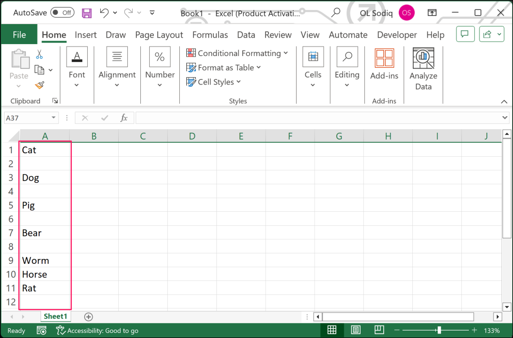
This method is best for deleting blank rows in Excel spreadsheets with only one column. Say you have the following set of data in Excel and want to get rid of the blank lines:
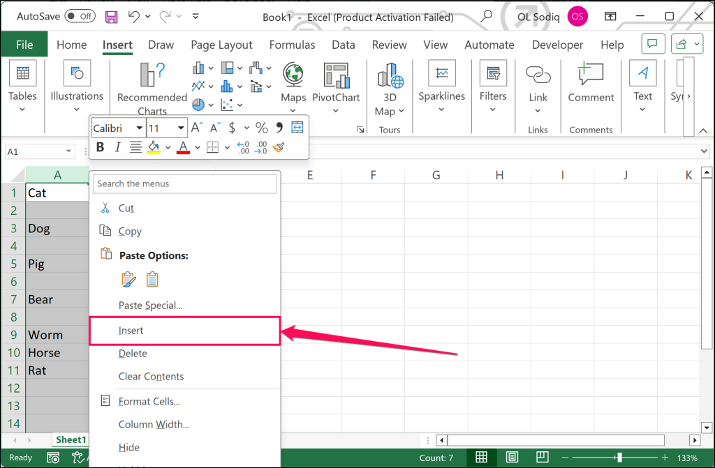
- Right-click the column header and select Insert to add a new column. This blank column will serve as an anchor/helper column to sort out blank rows in the original column.
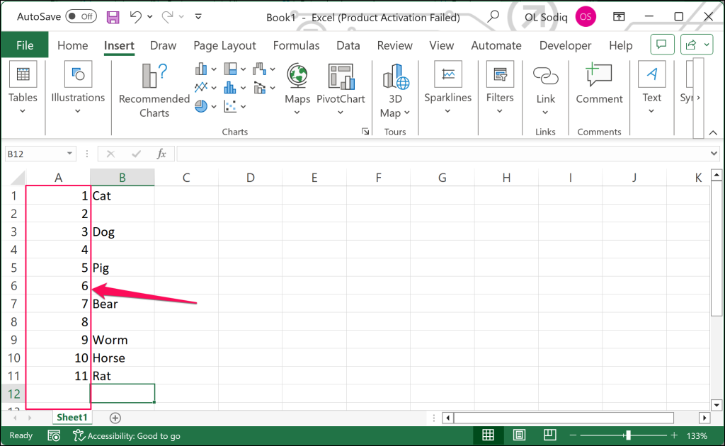
- Number the new column consecutively (1, 2, 3, 4, 5, etc.) from the first cell. Here’s what the sheet should look like before we sort the animal name column:
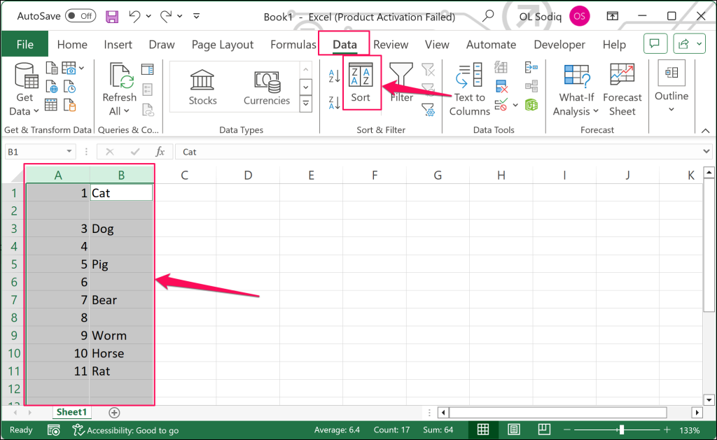
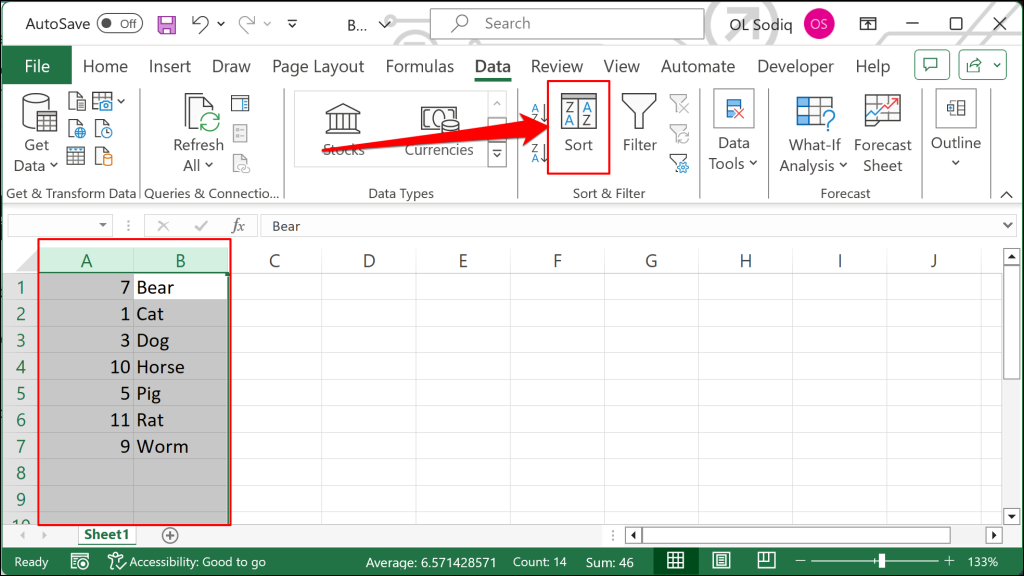
- Select both columns, open the Data tab on the ribbon, and select Sort.
- Open the Sort by drop-down menu and choose the column with empty/blank rows (“Column B” in our sample data). Select OK to proceed.
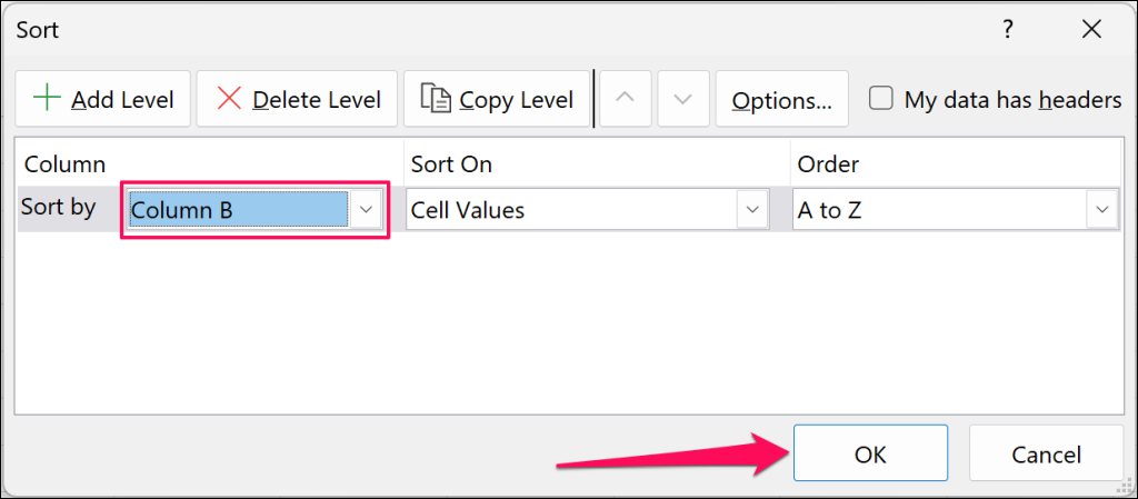
Note that you want to sort the column with the blank values. If multiple columns have empty values, choose the column you want to sort and select OK.
The sorting tool will reorder your column alphabetically, moving blank cells to the bottom. Before sorting, the order was “Cat, Dog, Pig, etc..” and now it’s “Bear, Cat, Cow, etc…”.
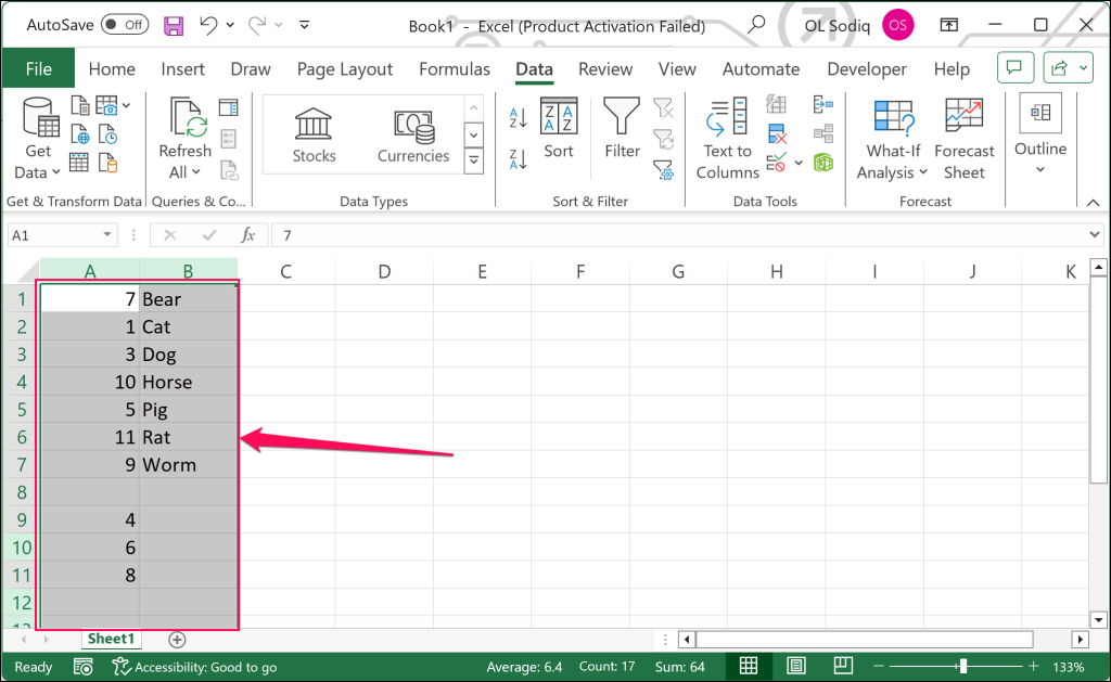
Select and delete the blank/empty rows. The next step is to restore cells in the column to their original order.
- Select both columns and choose Sort in the “Data” tab on the ribbon.
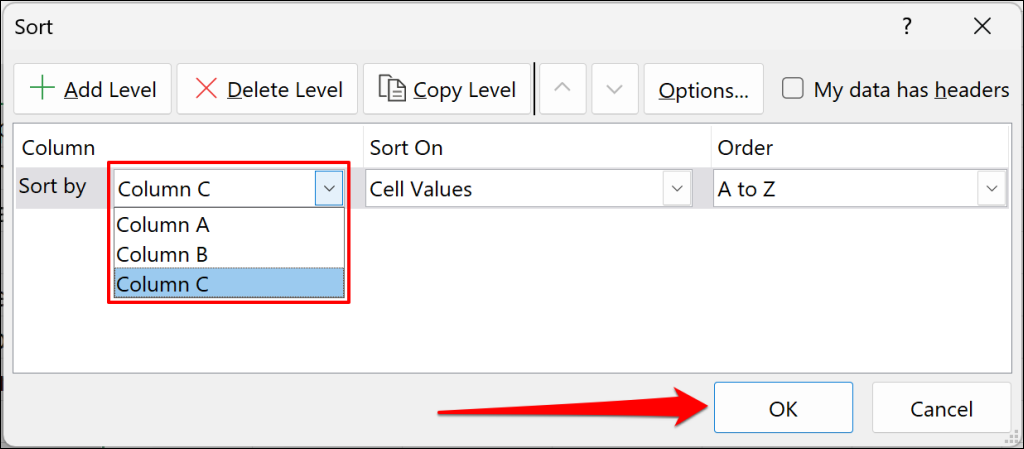
- Sort the data by the anchor/helper column and select OK. For our sample data, we’ll Sort by Column A.
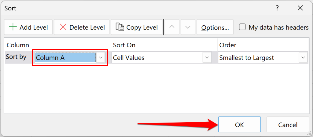
That’ll restore cells in the column to their original order. You can now delete the anchor/helper column.
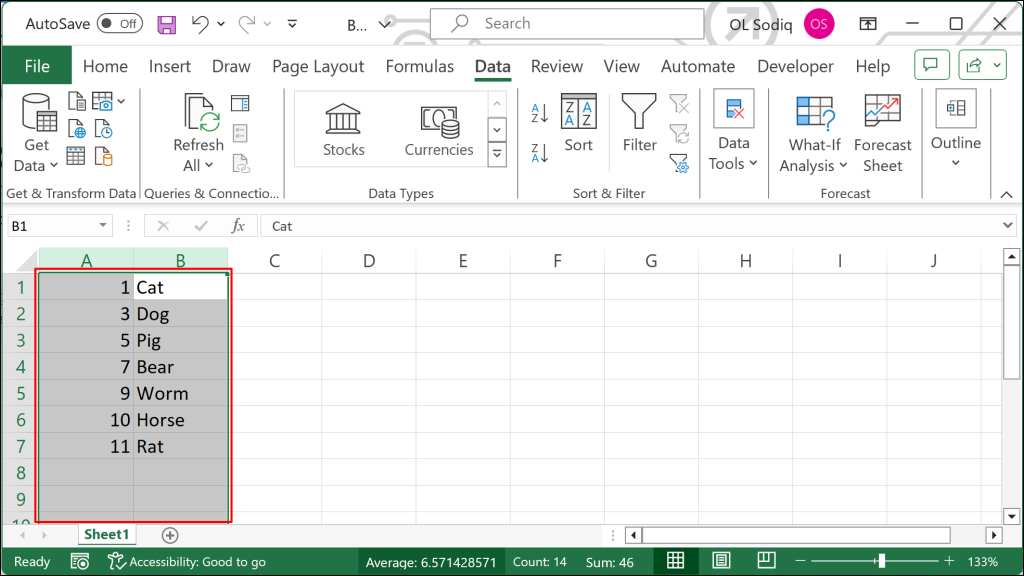
You can also use this method to delete rows with only one empty cell (or column). But what if you need to blank rows across multiple columns? The instructions in the next section will help you weed out blank or empty rows in a multi-column spreadsheet.
Delete Blank Row in Multiple Columns
We’ll use the sample data below (with several blank rows) to show how to use the Sort tool to delete blank rows in an Excel spreadsheet.
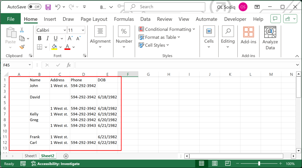
This spreadsheet has multiple blank rows and other rows with empty cells. Sorting the dataset by columns makes it easy to eliminate blank rows. Here’s how to get it done.
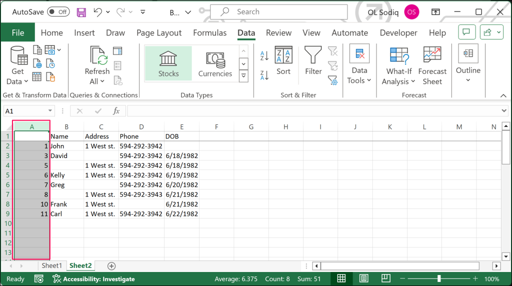
- First, add an anchor column to the left of the first column. Right-click the first column header and select Insert.
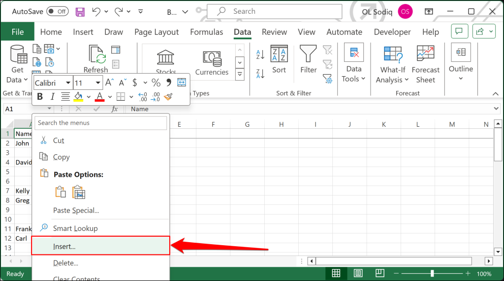
- Number cells in the anchor column (leaving out the header) consecutively.
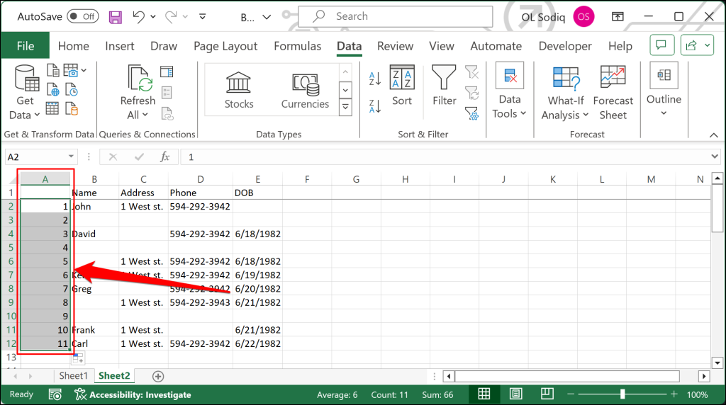
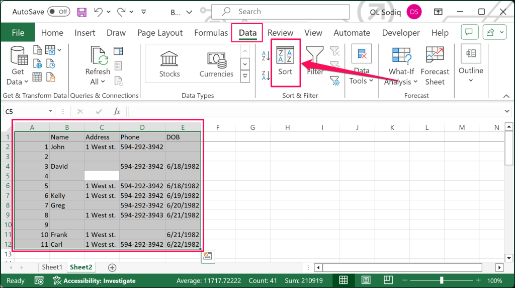
- Select all rows and columns (Ctrl + A), open the “Data” tab and select Sort.
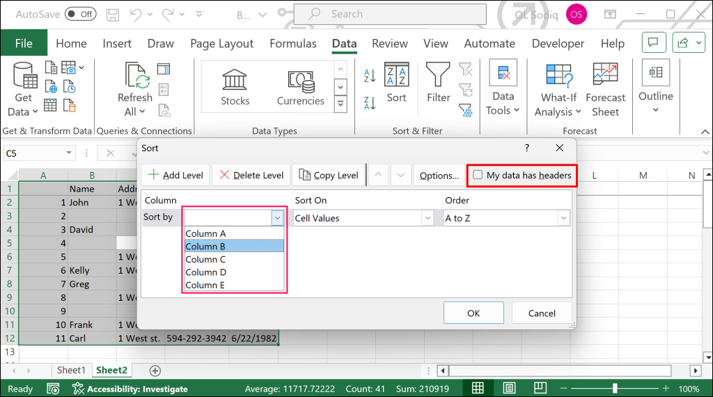
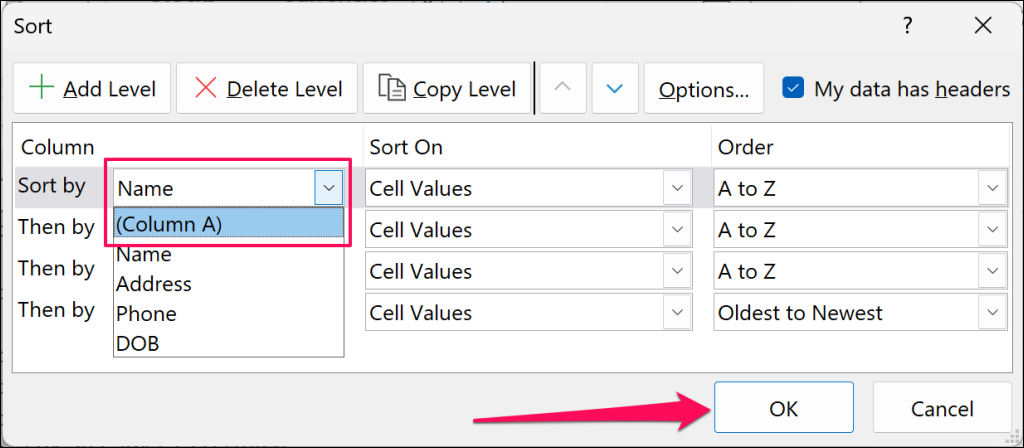
- Open the Sort by drop-down menu and select your dataset’s first column (not the anchor column. Check the My data has headers box if your worksheet has a fixed header.
The next step is creating a “Sort Level” for subsequent columns.
- Select the Add Level button in the top corner of the “Sort” dialog box.
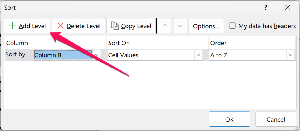
- Open the Then by drop-down menu for the newly-added level and select the subsequent column.
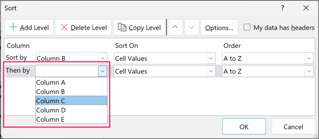
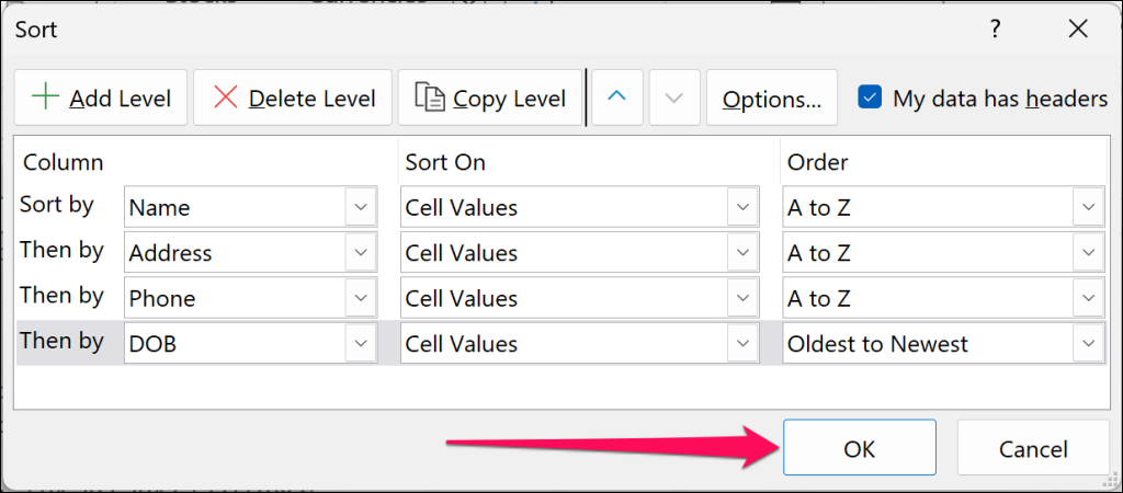
- Create new “Sort Levels” for all columns in your worksheet and add them to the “Then by” drop-down menu.

- Select OK to proceed.
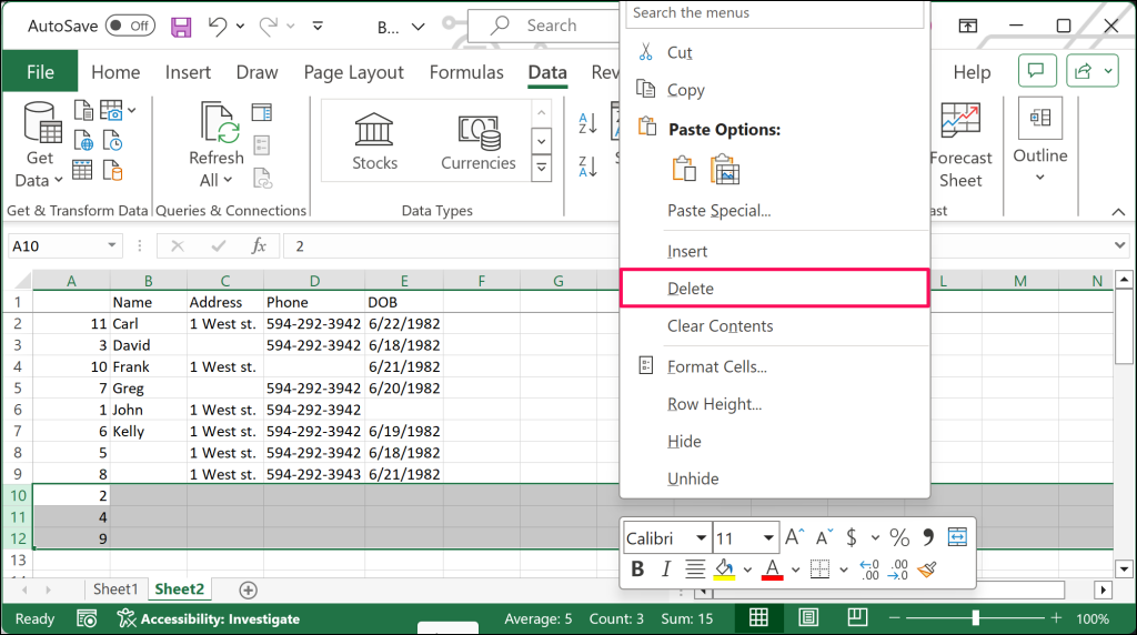
- Excel will move all blank rows to the bottom of the spreadsheet. Select the rows, right-click, and select Delete.
- Now, you want to restore the rows to their initial order. Select all columns (Ctrl + A) and Sort in the “Data” tab.
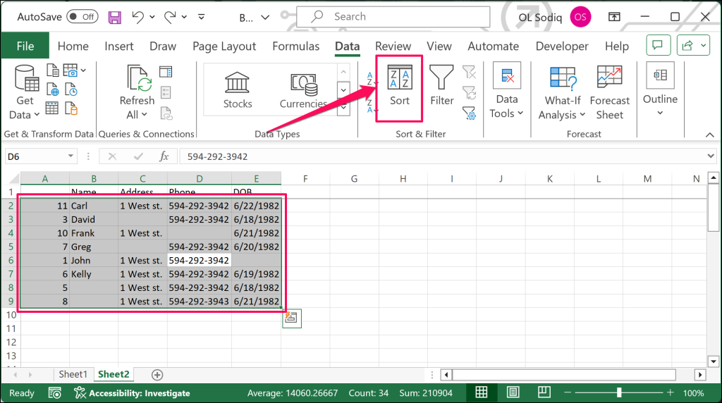
- Open the Sort by drop-down menu, choose the anchor column (Column A), and select OK.
Delete the anchor column (with numbers) to return your spreadsheet to its initial order.
How to Remove Blank Rows Using Filters
You can also use the Filter function to remove blank rows in an Excel spreadsheet. This method doesn’t involve adding an extra/anchor column to your dataset.
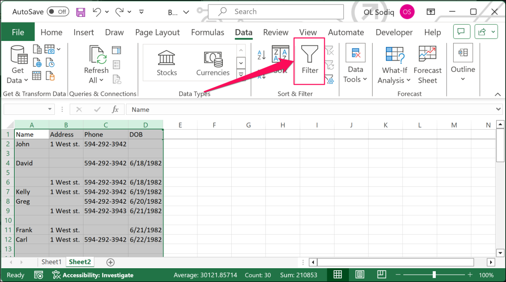
- Select the columns you want to inspect for blanks and select Filter in the “Data” tab.
- A drop-down arrow will appear next to each title in the header row. Select the drop-down icon next to the first column header/title. Uncheck Select All, select only the Blanks checkbox, and select OK.
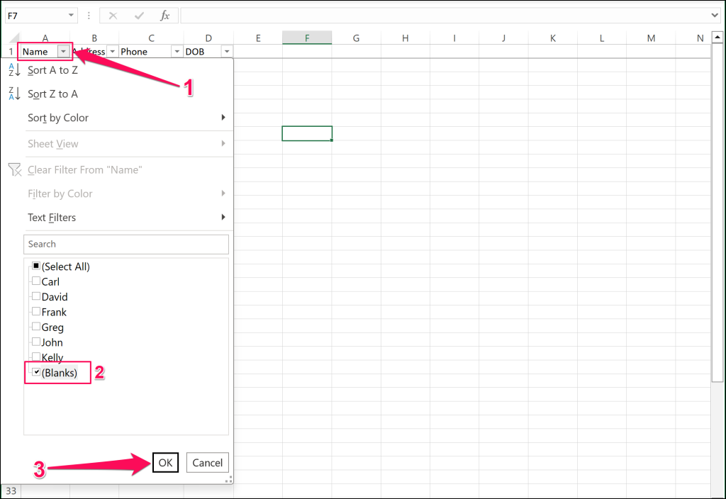
- Do the same for each column in the worksheet—open the title drop-down and select only the Blanks checkbox.
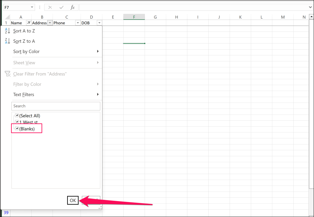
Note: If you get to a point where there are only blank rows showing, then you don’t have to filter for blanks for the remaining rows. You can proceed to remove blank rows in the spreadsheet.
- Excel will highlight the (row) number for empty rows in blue. Select those rows, right-click, and choose Delete Row on the context menu.
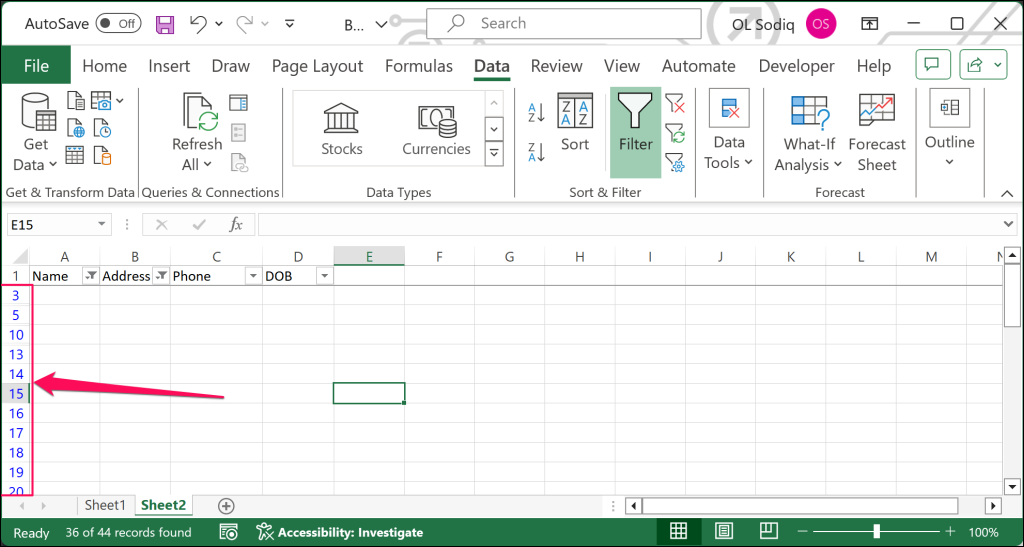
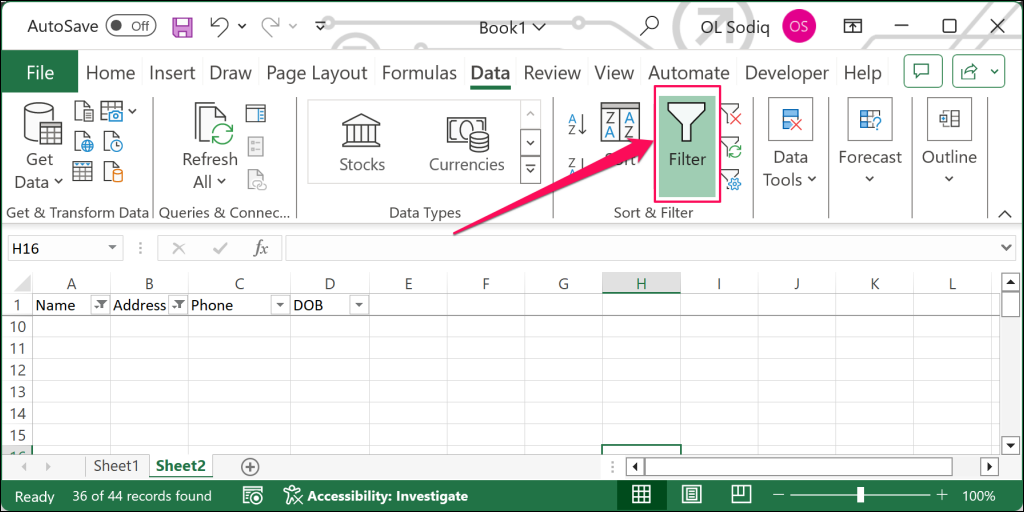
- After deleting the empty rows, select the Filter button in the “Data” tab. That’ll remove the filter and restore your spreadsheet without the blank rows.
How to Delete Any Blank Row or Cell
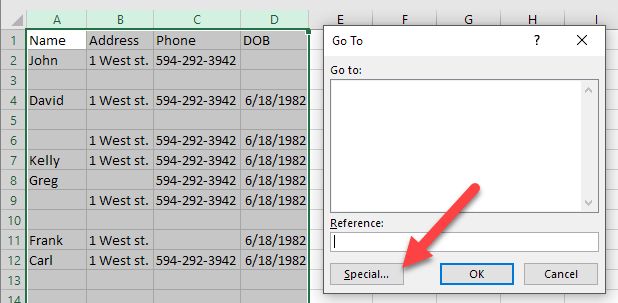
Use Excel’s “Go To” command to delete any row or cell with no value(s). This is useful when cleaning your dataset and removing any rows/columns with partial/incomplete data.
- Select all the data on the sheet and press the F5 key to open the Go To window. Select the Special button to proceed.
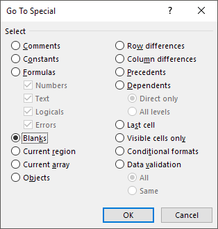
- Select Blanks from the options and select OK.
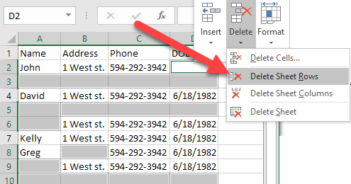
Excel will highlight all blank cells or rows in your worksheet.
- Select the Delete drop-down icon on the “Home” tab and choose Delete Sheet Rows.
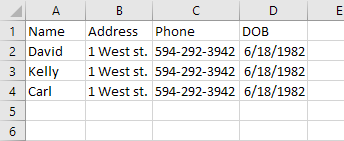
That’ll delete all rows or columns with a blank cell in your data.
Clean Up Your Excel Spreadsheet
Use the “Sort” tool to remove blank rows in an Excel spreadsheet with few (≤ 10) columns. Using the Filter tool is quicker and better if you work with a larger dataset.
