
You need to flip rows into columns (or columns into rows) in Excel, and the old Ctrl+Shift+Enter trick you found online isn’t working the way you expected. If you’re on Microsoft 365 or Excel 2021+, there’s a much simpler way to do it now, with no array gymnastics required.
Which method should you use?
There are two ways to transpose data in Excel, and the right one depends on whether you want the result to stay linked to the original data or just be a static copy.
| Method | Data stays linked? | Keeps formatting? | Best for |
|---|---|---|---|
| TRANSPOSE() formula | Yes, auto-updates | No | Live reports, dashboards |
| Paste Special | No, static copy | Yes | One-time layout changes |
Method 1: TRANSPOSE() Formula (Recommended for Live Data)
The TRANSPOSE() formula keeps the transposed data linked to the source. If you update the original, the transposed version updates automatically. On Microsoft 365 and Excel 2021+, you don’t need to pre-select a range or press Ctrl+Shift+Enter anymore. Just type the formula and press Enter.
If you’re on Microsoft 365 or Excel 2021+ (dynamic arrays)
- Click the cell where you want the transposed data to start (for example, G1).
- Type
=TRANSPOSE(A1:B6)replaceA1:B6with your actual source range. - Press Enter. Excel automatically spills the result into the surrounding cells.
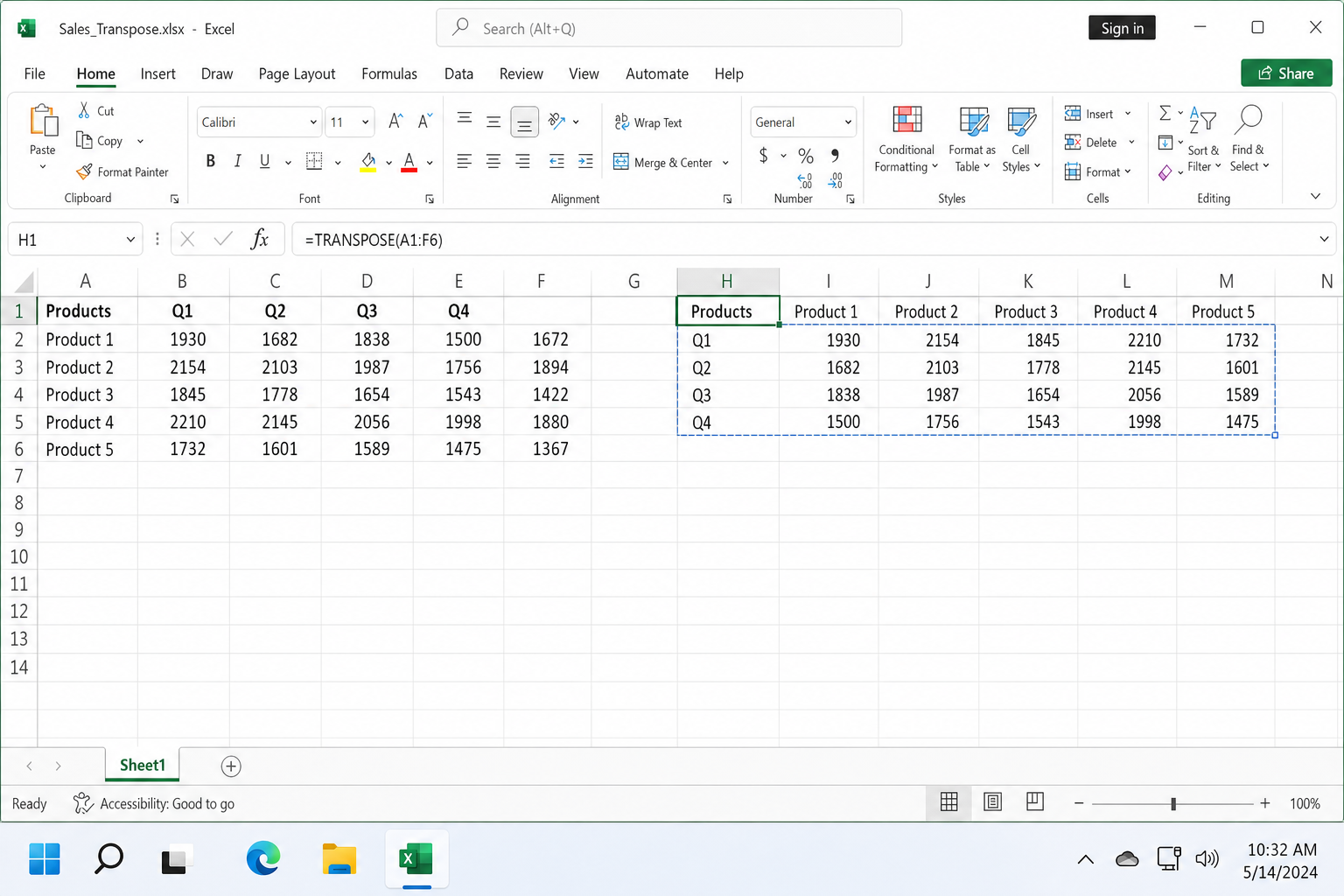
You should see the data appear across the neighboring cells instantly, with no pre-selection and no Ctrl+Shift+Enter. If you edit any cell in the original range, the transposed output updates to match.
Pro tip: If you see a #SPILL! error after pressing Enter, there are occupied cells blocking the spill range. Select those cells and press Delete to clear them, then the formula will resolve.
If you’re on Excel 2019 or older (legacy array formula)
Older Excel versions don’t support dynamic arrays, so you need to tell Excel upfront how many cells the result will occupy.
- Count the dimensions of your source range. If your source is 2 columns × 6 rows (e.g., A1:B6), the transposed result will be 6 columns × 2 rows.
- Select a blank area of that exact size, for example, select a 6×2 block starting at A12.
- Without clicking anywhere else, type
=TRANSPOSE(A1:B6)into the formula bar. - Press Ctrl+Shift+Enter instead of just Enter. Excel wraps the formula in curly braces:
{=TRANSPOSE(A1:B6)}.
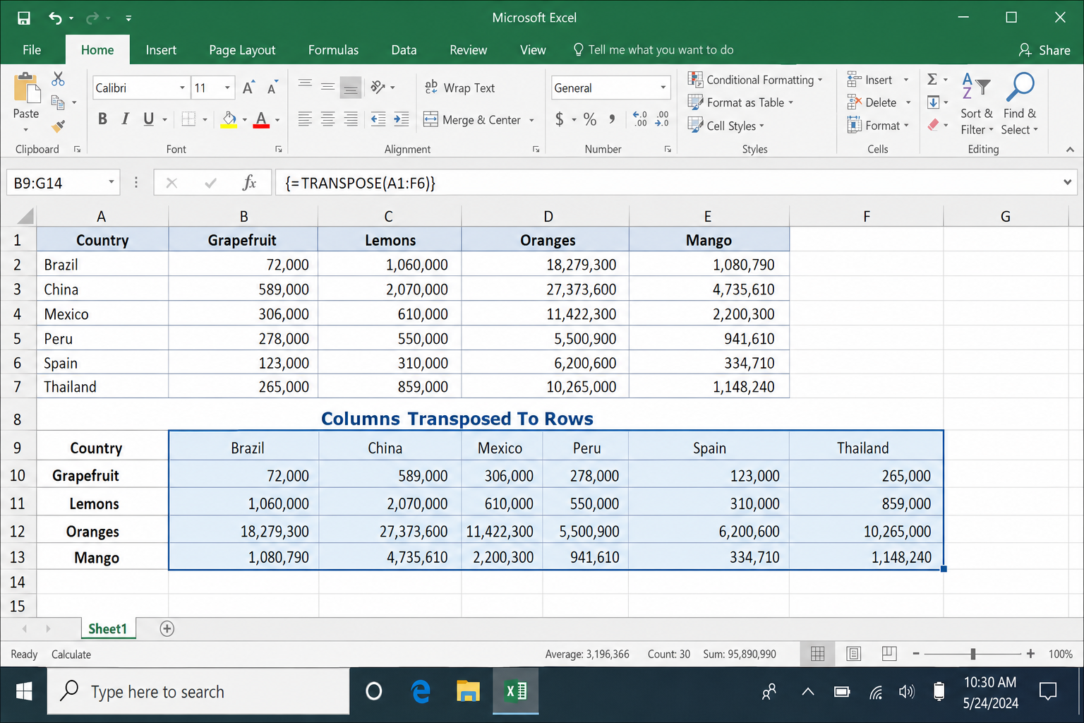
The curly braces confirm Excel treated this as an array formula. Don’t type the braces manually. They only appear when you use Ctrl+Shift+Enter.
Important: Because the transposed cells are linked to the source, deleting the original data will cause a reference error in the transposed range. If you need to delete the source, use Method 2 instead.
Method 2: Paste Special Transpose (Static Copy)
Paste Special gives you a clean, independent copy of the data in the new orientation, with no formulas and no link to the original. Formatting comes along for the ride, which the formula method doesn’t do.
- Select the data you want to transpose.
- Press Ctrl+C to copy it (don’t use Cut, Paste Special Transpose only works with Copy).
- Click the top-left cell of the empty area where you want the transposed data to appear.
- Right-click and choose Paste Special.
- Check the Transpose checkbox and click OK. Alternatively, hover over the paste icons in the right-click menu and click the Transpose icon (it looks like a small grid with a rotation arrow). Hovering gives you a live preview before you commit.
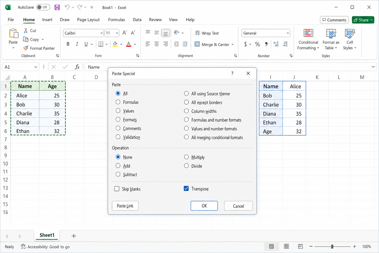
The transposed data is now completely independent. You can delete the original range without affecting it, and any changes you make to the original won’t carry over.
Common issues
| Problem | Cause | Fix |
|---|---|---|
| #SPILL! error | Cells in the spill range aren’t empty | Clear the cells: Home > Clear > Clear All |
| Formula shows in every cell | Legacy Excel, forgot Ctrl+Shift+Enter | Delete the result, re-select the range, re-enter with Ctrl+Shift+Enter |
| Transpose option is grayed out | Source data is an Excel Table | Convert to a range first: Table Design > Convert to Range |
| Formatting is missing after transpose | TRANSPOSE() formula doesn’t carry formats | Use Paste Special and check both Formats and Transpose |
| Transposed data doesn’t update | You used Paste Special (static) | Switch to the TRANSPOSE() formula method |
Conclusion
For most people on Microsoft 365, the =TRANSPOSE() formula is the better default. Type it in one cell, press Enter, and you’re done. Paste Special is still the right call when you need a one-time, formatting-intact copy that has no dependency on the original data. If you’re still on Excel 2019 or older, the Ctrl+Shift+Enter array method works fine, but it’s a solid reason to consider upgrading, as the dynamic array version is noticeably less painful.
If you run into other formula issues in Excel, check out our guide on Microsoft Excel formulas not working or calculating, and if you’re new to how Excel organizes data, our breakdown of Microsoft Excel workbooks and worksheets is a good place to start. You may also find it helpful to know how to find circular references in Microsoft Excel if your linked formulas start producing unexpected results.