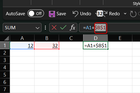
One feature that’s easy to overlook but is incredibly important for accurate calculations is “anchoring.” If you’ve ever copied an Excel formula, pasted it in a different cell, and saw unexpected results, anchoring might be the missing piece of the puzzle.
Let’s learn the difference between relative and absolute cell references and how to use them for anchoring cells in Microsoft Excel.
What Is Anchoring Cells in Excel?
Anchoring in Excel is like dropping an anchor from a ship. When you drop an anchor, your boat stays in place regardless of how the water moves. Similarly, when you anchor a cell in Excel, you ensure that the cell reference stays “fixed” even as you move and copy your formulas to different parts of your spreadsheet.
Anchoring cells can come in handy in many scenarios. For example, you’re working on a budget and have a cell containing the tax rate. As you calculate taxes for various items across your spreadsheet, you’ll want that tax rate to remain constant—not change as you drag your formula down a column or across a row.
Anchoring cells in Excel can save you from potential errors and simplify the process of using repetitive values across spreadsheets with lots of data.
Understanding Relative and Absolute Cell References
Understanding how anchor cells work requires knowledge about relative reference and absolute reference.
Think of relative references as Excel’s way of being adaptable. When you copy a relative reference in a formula to another cell, the reference changes based on its new location. You’re telling Excel to adjust the formula based on where you move it. For example, let’s say in A1 you use the =A2+10 formula, and then you copy this to B1, it will then become =B2+10 instead.
An absolute reference is the opposite. No matter where you copy your formula, an absolute reference ensures that part (or all) of the formula remains fixed on that specific cell. Using our tax reference from earlier, if you have the tax rate in A1 and you want to use this in various calculations, you can use $A$1 in your formulas. This tells Excel that no matter where you drag or copy the formula, always use the value in A1 for this part of the calculation.
So, as you may have guessed, you should anchor cells when you want to use an absolute reference.
How to Anchor Cells in Excel
Now that you understand the intricacies of anchoring a cell, here’s how to do it.
- Select the cell that contains the formula you’d like to anchor. This cell should have the special value or reference you don’t want to change, no matter where you use the formula next.
- In the formula bar at the top, add a $ (dollar sign) right before the column letter, the row number, or both, depending on what you want to keep constant. Alternatively, you can highlight the parts you want to anchor and press F4 (the keyboard shortcut). This will automatically add the dollar signs.
- Press Enter.
Your cell is now anchored. The anchored reference will remain the same when copying or moving this formula elsewhere.
Organize Your Data With the Right Anchors
Anchoring cells in Excel is a fundamental skill required for keeping spreadsheets accurate and consistent. By understanding the difference between relative and absolute references, you can control how formulas behave when moved or copied to different parts of the worksheet.
Related Posts
Marshall is a technical writer based in Tokyo, Japan. His bylines are found on VGKAMI, How-To Geek, PCWorld, Zapier, and many other online magazines. Read Marshall’s Full Bio


