Microsoft Excel may return an error when you input a value or try to perform an action that it fails to understand. There are several types of errors, and each error is associated with specific types of mistakes you might have made.
The #N/A error is a standard Excel error. It appears when you’ve referenced data incorrectly. For example, referenced data that doesn’t exist or exists outside of the lookup table, made a spelling error in the lookup value, or added an extra character in the lookup value (a comma, apostrophe, or even a space character).
Since the error occurs when you’ve incorrectly referenced a lookup value, it’s most commonly associated with lookup functions like LOOKUP, VLOOKUP, HLOOKUP, and the MATCH function. Let’s look at the reasons, an example, and some fixes for the #N/A error.
Reasons for #N/A Error
Following are the reasons that can cause a #N/A error on your worksheet:
- You’ve misspelled a lookup value (or inserted an extra space character)
- You’ve misspelled a value in the lookup table (or inserted an extra space character)
- The lookup range has been entered incorrectly into the formula
- You’ve used a different data type for the lookup value than the one that exists in the lookup table (i.e., used text instead of numbers)
- The lookup value you entered was not found in the lookup table
Example of #N/A Error
Let’s use the VLOOKUP function as an example to understand how you might end up with a #N/A error after using Excel functions like LOOKUP, HLOOKUP, or MATCH since they share a similar syntax structure.
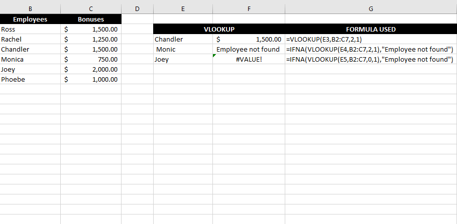
For instance, say you have a long list of employees and their bonuses listed in an Excel workbook.
You use the VLOOKUP formula, enter a relevant [lookup_value] for which you insert a cell reference (cell D4), define the [table_array] (A2:B7), and define [col_index_num] (2).
For the final argument called the [range_lookup], you should use 1 (or TRUE) to instruct Excel to obtain an exact match. Setting it to 2 (or FALSE) will instruct Excel to look for an approximate match, which can give you an incorrect output.
Suppose you’ve set up a formula for obtaining bonuses for a select few employees, but you misspell the lookup value. You’ll end up with a #N/A error because Excel won’t be able to find an exact match for the value in the lookup table.
So, what must you do to fix this error?
How to Fix #N/A Error
There are several ways for troubleshooting the #N/A error, but the fixes can primarily be categorized into two approaches:
- Correcting the inputs
- Trapping the error
Correcting the inputs
Ideally, you should identify the cause of the error using the reasons listed previously in this tutorial. Fixing the cause will ensure that you’re not just getting rid of the error but also getting the correct output.
You should start by using the reasons listed in this guide as a checklist. Doing this will help you find the incorrect input that you need to fix to eliminate the error. For example, it could be a misspelled value, an extra space character, or values with an incorrect data type in the lookup table.
Trapping the error
Alternatively, if you want to just eliminate errors from your worksheet without bothering with individually checking for mistakes, you can use several Excel formulas. Some functions have been created specifically to trap errors, while others can help you construct a logical syntax using multiple functions to eliminate errors.
You can trap the #N/A error using one of the following functions:
- IFERROR Function
- IFNA Function
- A Combination of ISERROR Function and IF Function
- TRIM Function
1. IFERROR Function
The IFERROR function was created with the sole purpose of changing the output for a cell that returns an error.
Using the IFERROR function allows you to enter a specific value that you want a cell to show instead of an error. For instance, if you have a #N/A error in cell E2 when using VLOOKUP, you can nest the entire formula into an IFERROR function, like so:
IFERROR(VLOOKUP(E4,B2:C7,2,1),“Employee not found”
If the VLOOKUP function results in an error, it will automatically display the text string “Employees not found” instead of the error.
You can also use an empty string by simply inserting two quotation marks (“”) if you want to display a blank cell when the formula returns an error.
Note that the IFERROR function works for all errors. So, for instance, if the formula you’ve nested inside the IFERROR function returns a #DIV error, IFERROR will still trap the error and return the value in the last argument.
2. IFNA Function
The IFNA function is a more specific version of the IFERROR function but works exactly the same way. The only difference between the two functions is that the IFERROR function traps all errors, while the IFNA function only traps #N/A errors.
For instance, the following formula will work if you have a VLOOKUP #N/A error, but not for a #VALUE error:
IFNA(VLOOKUP(E4,B2:C7,2,1),“Employee not found”
3. A Combination of the ISERROR Function and the IF Function
Another way to trap an error is to use the ISERROR function along with the IF function. It essentially works like the IFERROR function, in that it relies on the ISERROR function to detect an error, and the IF function to render output based on a logical test.
The combination works with all errors like the IFERROR function, not just the #N/A function. Here’s an example of what the syntax will look like when trapping an Excel VLOOKUP #N/A error with the IF and ISERROR functions:
=IF(ISERROR(VLOOKUP(E4,B2:C7,2,1)),VLOOKUP(E4,B2:C8,2,1),”Employee not found”)
4. TRIM Function
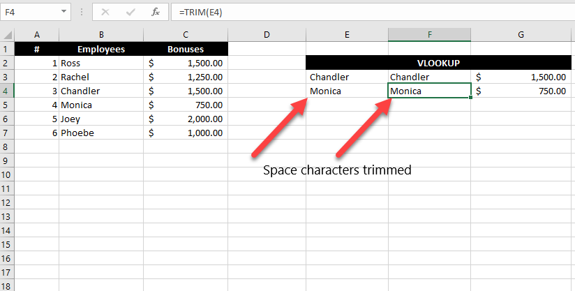
We discussed earlier that a space character inserted inadvertently in the lookup value can result in a #N/A error. However, if you have a long list of lookup values already populated into your worksheet, you can use the TRIM function instead of removing the space character from each lookup value individually.
First, create another column to trim leading and trailing spaces in the names using the TRIM function:
Then, use the new column of names as the lookup values in the VLOOKUP function.
Fix #N/A Error in Macros
There’s no specific formula or shortcut you can use to fix #N/A errors in a macro. Since you likely added several functions into your macro when you created it, you’ll need to check the arguments used for each function and verify if they’re correct to fix an #N/A error in a maco.
#N/A Errors Fixed
Fixing #N/A errors isn’t that difficult once you understand what causes them. If you’re not too concerned about the output and just don’t want a formula to result in an error, you can use functions like IFERROR and IFNA to easily tackle the #N/A error.


