How to Show Negative Numbers as Red in Excel

When you use Microsoft Excel for things like a household budget, business financials, or product inventory, you may end up with negative numbers at times. To make those less-than-zero numbers pop, here’s how to make them a red color.

We’ll explain three methods for showing negative numbers as red in Excel. Use whichever you’re most comfortable with or works best for your sheet.

Format the Cells for Negative Red Numbers

For the easiest way to format your negative numbers red, open your workbook to the spreadsheet and follow these steps.

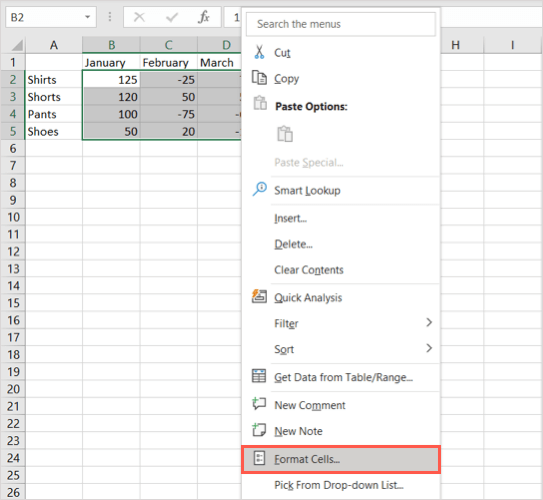
1. Select the cells you want to format.
2. For the entire sheet use the Select All button (triangle) on the top left of the sheet between column A and row 1. You should see your whole sheet shaded.
3. For particular cells, drag your cursor through them or hold Ctrl as you select each one.
4. Right-click any of the selected cells and pick Format Cells to open the Format Cells dialog box.

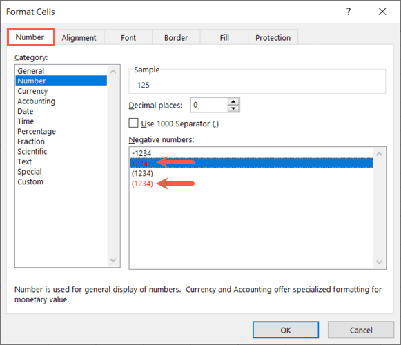
5. On the Number tab, choose the format type in the Category list on the left. You can format negative Numbers and Currency in a red font color.
6. On the right, pick one of the two red options in the Negative numbers box. You can use just red for the number or place the number in parentheses and make it red.

7. Select OK at the bottom to apply the change.

You should then see any negative numbers in your selected cells turn red while the positive numbers remain the same.

Create a Custom Format for Negative Red Numbers

While the above is the simplest way to turn negative values red, you may not like the two choices you have. Perhaps you’d like to keep the negative sign (-) in front of the number. For this, you can create a custom number format.

1. Select the cells or sheet where you want to apply the formatting as described in Step 1 above.
2. Right-click any of the selected cells and pick Format Cells.
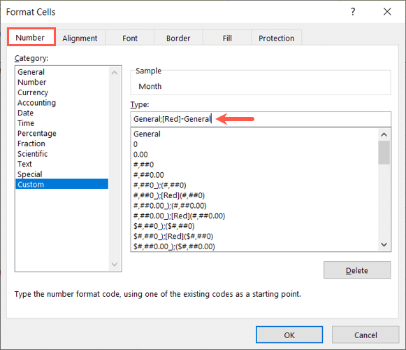
3. On the Number tab, choose Custom in the Category list on the left.
4. In the Type box on the right enter: General;[Red]-General.

5. Select OK to apply the formatting.

Now you’ll see your worksheet update and turn negative numbers red while retaining the minus signs in front of the numbers.

Use Conditional Formatting for Negative Red Numbers

Another option to make negative numbers red in Excel is with a conditional formatting rule. The advantage to this method is that you can choose the shade of red you want or apply additional formatting such as changing the cell color or making the font bold or underlined.

1. Select the data set where you want to apply the formatting or the entire sheet as described above.
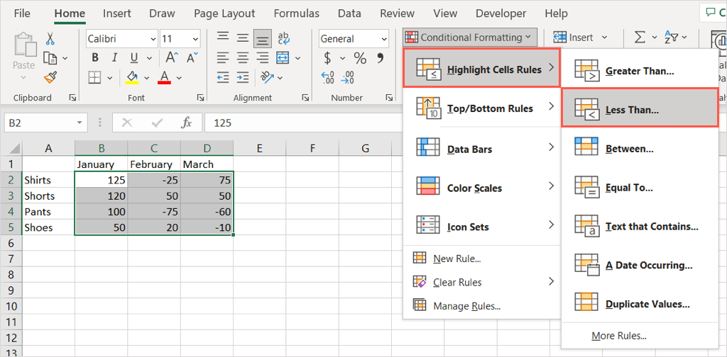
2. Go to the Home tab and select the Conditional Formatting drop-down menu in the Styles section of the ribbon.
3. Move your cursor to Highlight Cell Rules and pick Less Than in the pop-out menu.

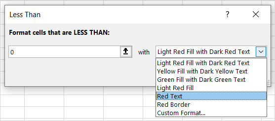
4. In the small box that appears enter a zero (0) in the Format cells that are LESS THAN box.
5. In the drop-down list to the right, pick Red Text.

6. Alternatively, you can choose another quick format from the list or select Custom Format to use your own. If you pick the latter, go to the Font tab and use the Color drop-down box to choose the shade of red you want. You can use More Colors to see additional options. Apply any other formatting you’d like to the cells with negative numbers.

7. Select the OK button and OK again if you picked a custom option.

You’ll then see your selected cells update to display negative numbers in a red font color and any other formatting you chose.

With built-in ways to show negative numbers red in Excel, you can make sure those numbers stand out from the rest in your sheet.

For more Excel tutorials, look at ways to convert text to numbers in your spreadsheet.