The three most commonly used formulas in Excel that perform simple mathematical calculations are COUNT, SUM and AVERAGE. Whether you are managing a financial budget in Excel or simply keeping track of your next vacation, you’ve probably used one of these functions before.
In this article, we’re going to go through the basics of these three functions and their relevant and useful counterparts: COUNTIFS, SUMIFS and AVERAGEIFS.
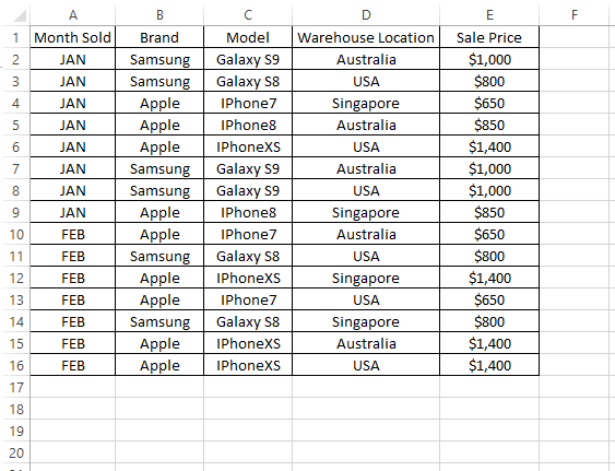
Let’s say we are starting a new online business selling mobile phones and we have a sheet that lists the sales that we have made in the first two months. Download example Excel spreadsheet here.
Excel COUNT, SUM and AVERAGE
To know how many mobile phones that we have sold, we can quickly use the COUNT formula as shown below:
=COUNT(E2:E16)
On the other hand, to get the total amount of sales that we have made, we can use the SUM formula as shown below:
=SUM(E2:E16)
Lastly, to find out the average sales that we made for all phones, we can use the AVERAGE formula as below:
=AVERAGE(E2:E16)
The result should be as below:
COUNT, SUM and AVERAGE formulas will only work for records where the cell value is in number format. Any record within the formula range (i.e. E2:E16 in this example) not in the number format will be ignored.
So, please ensure that all cells within the COUNT, SUM and AVERAGE formula are all formatted as Number, not Text. Try to use the same formula, but with E:E as the range instead of E2:E16. It will return the same result as before because it ignores the header (i.e. Sale Price), which is in text format.
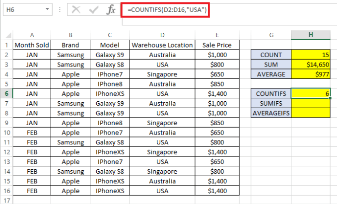
Now, what if we want to know number of sales, total amount of sales and the average amount of sales per phone, just for those sold in USA? This is where COUNTIFS, SUMIFS and AVERAGEIFS play an important role. Observe the formula below:
COUNTIFS
Formula breakdown:
- =COUNTIFS( – The “=” indicates the beginning of a formula in the cell and COUNTIFS is the first part of the Excel function that we are using.
- D2:D16 – Refers to range of data to check to see if it satisfies the criteria to be included in the count formula.
- “USA” – Criteria to look for in the data range specified (D2:D16)
- ) – Closing bracket indicating the end of the formula.
The formula returns 6 which is the number of sales for products shipped from the USA warehouse.
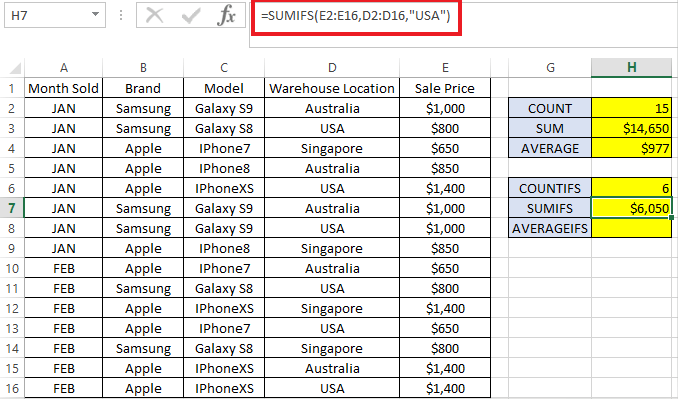
SUMIFS
Formula breakdown:
- =SUMIFS( – The “=” indicates the beginning of the formula again.
- E2:E16 – Refers to range of data that we would like to total, i.e. sale price in our example.
- D2:D16 – Refers to range of data to check to see if it satisfies the criteria to be included in the total amount.
- “USA” – Criteria to look for in the data range specified (D2:D16)
- ) – Closing bracket indicating the end of the formula.
The formula shows $6,050 total sales that were made for products shipped from the USA warehouse.
AVERAGEIFS
Formula breakdown:
- =AVERAGEIFS( – The “=” indicate the beginning of formula.
- E2:E16 – Refers to range of data that we would like to average. In this example, we want to get the average amount of sales for all phones sold in the USA.
- D2:D16 – Refers to range of data to check to see if it satisfies the criteria to be included in the average formula.
- “USA” – Criteria to look for in the data range specified
- ) – Closing bracket indicating the ends of the formula.
The formula shows we sold the product for around $1,008 per phone in USA.
All three formula can take more than one criteria. For example if we want to know the same figures (i.e. COUNT, SUM and AVERAGE) for products sold in USA, but specifically only for the Samsung brand, we just need to add the data range to be checked followed by its criteria.
Please see example below where a second criteria is added to the initial criteria checks. (Blue text indicates the first criteria and red indicates the second criteria)
=COUNTIFS(D2:D16,"USA", B2:B16,"Samsung")

=SUMIFS(E2:E16,D2:D16,"USA", B2:B16,"Samsung")

=AVERAGEIFS(E2:E16,D2:D16,"USA", B2:B16,"Samsung")
You will notice that Excel also has COUNTIF, SUMIF and AVERAGEIF formulas without the suffix “S”. Those are used similar to COUNTIFS, SUMIFS and AVERAGEIFS. However, those without the suffix “S” in the formula have the limitation of only allowing one criteria per formula.
As the syntax is slightly different, I would recommend using COUNTIFS, SUMIFS and AVERAGEIFS only as it can be used for either one criteria or more, if necessary. Enjoy!


