Use Dynamic Range Names in Excel for Flexible Dropdowns

Excel spreadsheets often include cell dropdowns to simplify and/or standardize data entry.  These dropdowns are created using the data validation feature to specify a list of allowable entries.

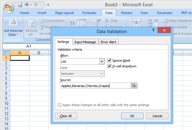
To set up a simple dropdown list, select the cell where data will be entered, then click Data Validation (on the Data tab), select Data Validation, choose List (under Allow:), and then enter the list items (separated by commas) in the Source: field (see Figure 1).

In this type of basic dropdown, the list of allowable entries is specified within the data validation itself; therefore, to make changes to the list, the user must open and edit the data validation.  This may be difficult, however, for inexperienced users, or in cases where the list of choices is lengthy.

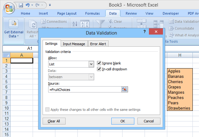
Another option is to place the list in a named range within the spreadsheet, and then specify that range name (prefaced with an equal sign) in the Source: field of the data validation (as shown in Figure 2).

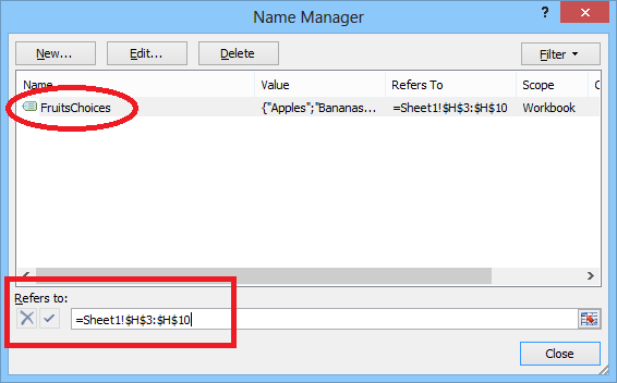
This second method makes it easier to edit the choices in the list, but adding or removing items can be problematic.  Since the named range (FruitChoices, in our example) refers to a fixed range of cells ($H$3:$H$10 as shown), if more choices are added to the cells H11 or below, they will not show up in the dropdown (since those cells are not part of the FruitChoices range).

Likewise if, for example, the Pears and Strawberries entries are erased, they will no longer appear in the dropdown, but instead the dropdown will include two “empty” choices since the dropdown still references the entire FruitChoices range, including the empty cells H9 and H10.

For these reasons, when using a normal named range as the list source for a dropdown, the named range itself must be edited to include more or fewer cells if entries are added or deleted from the list.

A solution to this problem is to use a dynamic range name as the source for the dropdown choices.  A dynamic range name is one that automatically expands (or contracts) to exactly match the size of a block of data as entries are added or removed.  To do this, you use a formula, rather than a fixed range of cell addresses, to define the named range.

How to Setup a Dynamic Range in Excel

A normal (static) range name refers to a specified range of cells ($H$3:$H$10 in our example, see below):

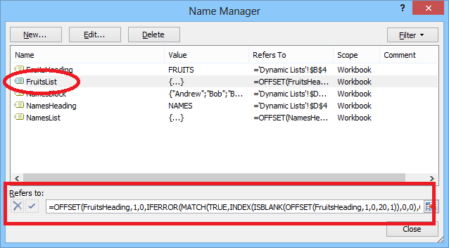
But a dynamic range is defined using a formula (see below, taken from a separate spreadsheet which uses dynamic range names):

Before we get started, make sure you download our Excel example file (sort macros have been disabled).

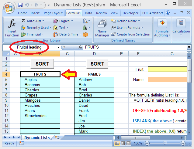
Let’s examine this formula in detail.  The choices for Fruits are in a block of cells directly below a heading (FRUITS).  That heading is also assigned a name: FruitsHeading:

The entire formula used to define the dynamic range for the Fruits choices is:

=OFFSET(FruitsHeading,1,0,IFERROR(MATCH(TRUE,INDEX(ISBLANK(OFFSET(FruitsHeading,1,0,20,1)),0,0),0)-1,20),1)

FruitsHeading refers to the heading that is one row above the first entry in the list.  The number 20 (used two times in the formula) is the maximum size (number of rows) for the list (this can be adjusted as desired).

Note that in this example, there are only 8 entries in the list, but there are also empty cells below these where additional entries could be added.  The number 20 refers to the entire block where entries can be made, not to the actual number of entries.

Now let’s break down the formula into pieces (color-coding each piece), to understand how it works:

=OFFSET(FruitsHeading,1,0,IFERROR(MATCH(TRUE,INDEX(ISBLANK(OFFSET(FruitsHeading,1,0,20,1)),0,0),0)-1,20),1)

The “innermost” piece is OFFSET(FruitsHeading,1,0,20,1).  This references the block of 20 cells (underneath the FruitsHeading cell) where choices may be entered.  This OFFSET function basically says: Start at the FruitsHeading cell, go down 1 row and over 0 columns, then select an area that is 20 rows long and 1 column wide.  So that gives us the 20-row block where the Fruits choices are entered.

The next piece of the formula is the ISBLANK function:

=OFFSET(FruitsHeading,1,0,IFERROR(MATCH(TRUE,INDEX(ISBLANK(the above),0,0),0)-1,20),1)

Here, the OFFSET function (explained above) has been replaced with “the above” (to make things easier to read).  But the ISBLANK function is operating on the 20-row range of cells that the OFFSET function defines.

ISBLANK then creates a set of 20 TRUE and FALSE values, indicating whether each of the individual cells in the 20-row range referenced by the OFFSET function is blank (empty) or not.  In this example, the first 8 values in the set will be FALSE since the first 8 cells are not empty and the last 12 values will be TRUE.

The next piece of the formula is the INDEX function:

=OFFSET(FruitsHeading,1,0,IFERROR(MATCH(TRUE,INDEX(the above,0,0),0)-1,20),1)

Again, “the above” refers to the ISBLANK and OFFSET functions described above.  The INDEX function returns an array containing the 20 TRUE / FALSE values created by the ISBLANK function.

INDEX is normally used to pick a certain value (or range of values) out of a block of data, by specifying a certain row and column (within that block).  But setting the row and column inputs to zero (as is done here) causes INDEX to return an array containing the entire block of data.

The next piece of the formula is the MATCH function:

=OFFSET(FruitsHeading,1,0,IFERROR(MATCH(TRUE,the above,0)-1,20),1)

The MATCH function returns the position of the first TRUE value, within the array that’s returned by the INDEX function.  Since the first 8 entries in the list are not blank, the first 8 values in the array will be FALSE, and the ninth value will be TRUE (since the 9^th row in the range is empty).

So the MATCH function will return the value of 9.  In this case, however, we really want to know how many entries are in the list, so the formula subtracts 1 from the MATCH value (which gives the position of the last entry).  So ultimately, MATCH(TRUE,the above,0)-1 returns the value of 8.

The next piece of the formula is the IFERROR function:

=OFFSET(FruitsHeading,1,0,IFERROR(the above,20),1)

The IFERROR function returns an alternate value, if the first value specified results in an error.  This function is included since, if the entire block of cells (all 20 rows) are filled with entries, the MATCH function will return an error.

This is because we’re telling the MATCH function to look for the first TRUE value (in the array of values from the ISBLANK function), but if NONE of the cells are empty, then the entire array will be filled with FALSE values.  If MATCH cannot find the target value (TRUE) in array it is searching, it returns an error.

So, if the entire list is full (and therefore, MATCH returns an error), the IFERROR function will instead return the value of 20 (knowing that there must be 20 entries in the list).

Finally, OFFSET(FruitsHeading,1,0,the above,1) returns the range we are actually looking for:  Start at the FruitsHeading cell, go down 1 row and over 0 columns, then select an area that is however many rows long as there are entries in the list (and 1 column wide).  So the entire formula together will return the range that contains only the actual entries (down to the first empty cell).

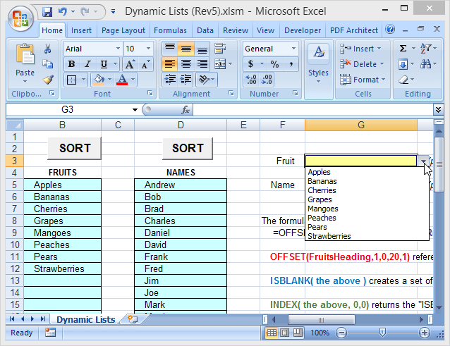
Using this formula to define the range that is the source for the dropdown means you can freely edit the list (adding or removing entries, as long as the remaining entries start at the top cell and are contiguous) and the dropdown will always reflect the current list (see Figure 6).

The example file (Dynamic Lists) that’s been used here is included and is downloadable from this website. The macros don’t work, however, because WordPress doesn’t like Excel books with macros in them.

As an alternative to specifying the number of rows in the list block, the list block can be assigned its own range name, which can then be used in a modified formula.  In the example file, a second list (Names) uses this method.  Here, the entire list block (underneath the “NAMES” heading, 40 rows in the example file) is assigned the range name of NameBlock.  The alternate formula for defining the NamesList is then:

=OFFSET(NamesHeading,1,0,IFERROR(MATCH(TRUE,INDEX(ISBLANK(NamesBlock),0,0),0)-1,ROWS(NamesBlock)),1)

where NamesBlock replaces OFFSET(FruitsHeading,1,0,20,1) and ROWS(NamesBlock) replaces the 20 (number of rows) in the earlier formula.

So, for dropdown lists which can be easily edited (including by other users who may be inexperienced), try using dynamic range names!  And note that, although this article has been focused on dropdown lists, dynamic range names can be used anywhere you need to reference a range or list that can vary in size. Enjoy!