When to Use Index-Match Instead of VLOOKUP in Excel

We'll show you with an example

Written by: Aseem Kishore, Twitter: @akishore
Posted on: November 30th, 2018 in: Office Tips

For those of you who are well-versed in Excel, you are most likely very familiar with the VLOOKUP function. The VLOOKUP function is used to find a value in a different cell based on some matching text within the same row.

If you are still new to VLOOKUP function, you can check out my previous post on how to use VLOOKUP in Excel.

Table of Contents

As powerful as it is, VLOOKUP has a limitation on how the matching reference table needs to be structured in order for the formula to work.

This article will show you the limitation where VLOOKUP cannot be used and introduce another function in Excel called INDEX-MATCH that can solve the issue.

INDEX MATCH Excel Example

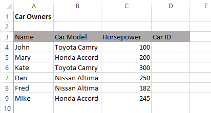
Using the following example Excel spreadsheet, we have a list of car owners name and the car name. In this example, we will be trying to grab the Car ID based on the Car Model listed under multiple owners as shown below:

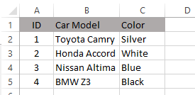
On a separate sheet called CarType, we have a simple car database with the ID, Car Model and Color.

With this table setup, the VLOOKUP function can only work if the data that we want to retrieve is located on the column to the right of what we are trying to match (Car Model field).

In other words, with this table structure, since we are trying to match it based on the Car Model, the only information that we can get is Color (Not ID as the ID column is located to the left of the Car Model column.)

This is because with VLOOKUP, the lookup value must appear in the first column and the lookup columns have to be to the right. None of those conditions are met in our example.

The good news is, INDEX-MATCH will be able to help us in achieving this. In practice, this is actually combining two Excel functions that can work individually: INDEX function and MATCH function.

However, for the purpose of this article, we will only talk about the combination of the two with the aim of replicating the function of VLOOKUP.

The formula can seem to be a little bit long and intimidating at first. However, once you have used it several times, you will learn the syntax by heart.

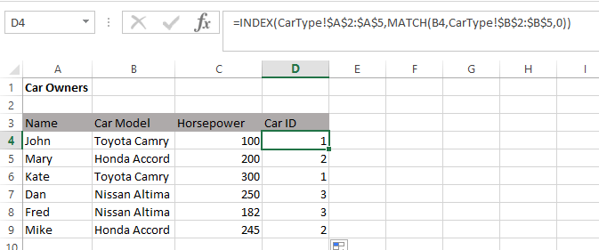
This is the full formula in our example:

=INDEX(CarType!$A$2:$A$5,MATCH(B4,CarType!$B$2:$B$5,0))

Here is the breakdown for each section

=INDEX( – The “=” indicates the beginning of formula in the cell and INDEX is the first part of the Excel function that we are using.

CarType!$A$2:$A$5 – the columns on sheet CarType where the data we would like to retrieve is contained. In this example, the ID of each Car Model.

MATCH( – The second part of the Excel function that we are using.

B4 – The cell that contain search text that we are using (Car Model).

CarType!$B$2:$B$5 – The columns on sheet CarType with the data which we will use to match against the search text.

0)) – To indicate that the search text has to exactly match with the text in the matching column (i.e. CarType!$B$2:$B$5). If the exact match is not found, the formula returns #N/A.

Note: remember the double closing bracket at the end of this function “))” and the commas between the arguments.

Personally I have moved away from VLOOKUP and now use INDEX-MATCH as it is capable of doing more than VLOOKUP.

The INDEX-MATCH functions also have other benefits as compared to VLOOKUP:

Faster Calculations

When we are working with large datasets where the calculation itself can take a long time due to many VLOOKUP functions, you will find that once you replace all of those formulas with INDEX-MATCH, the overall calculation will be compute faster.

No Need to Count Relative Columns

If our reference table is having the key text that we want to search in column C and the data that we need to get is in column AQ, we will need to know/count how many columns are between column C and column AQ when using VLOOKUP.

With the INDEX-MATCH functions, we can directly select the index column (i.e column AQ) where we need to get the data and select the column to be matched (i.e. column C).