How to Use Absolute References in Excel

Most people are familiar with using relative references in Excel. This is because cell references in Excel spreadsheets default to the relative reference method.

However, there are times when relative references get annoying. It will change cell references any time you copy cells or fill columns and rows. If you don’t want references to change, you’ll need to go with absolute references or mixed references (including relative and absolute references).

In an absolute reference, both the column and row references are “locked,” so neither of those change when you copy or fill from that cell.

This article will look at how you can use absolute references to make Excel behave the way you want with data.

How Relative References Work in Excel

When you enter values into an Excel spreadsheet, each cell has a specific letter and number assigned to it. This represents the column and row of that cell.

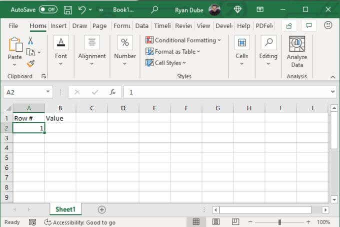
For example, the value of “1” in the spreadsheet below is in column A and row 2. So the “reference” to this cell is A2.

If you want to perform a calculation in the next cell based on this cell, by adding 1 to it, you will write the following formula:

=A2+1

This formula will insert the value from A2 into the formula, calculate it, and then output the result into the cell where this formula is.

When you press Enter, you’ll see the result.

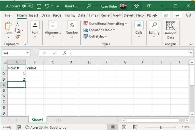
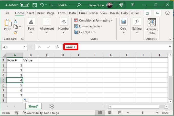
With relative referencing, you don’t have to type this formula into every other cell. All you have to do is drag the corner of the cell with the original formula down as far as you’d like. 

In the next cell, the reference to A2 will become A3. In the cell below that, A3 will become A4. In other words, Excel knows that you want to add 1 to the previous cell, so Excel updates the number (the row reference) accordingly as you drag down.

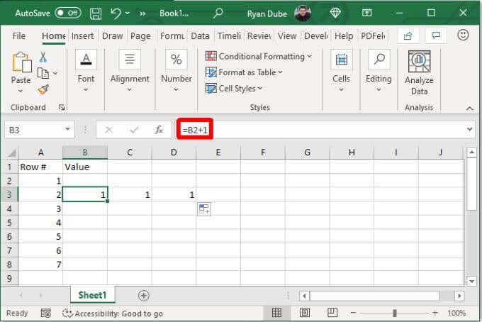
This works in the same way if you drag the formula across columns. Instead of updating the number, Excel will update the latter part of the reference (the column) to always reference the cell above it.

The column to the right contains B2, to the right of that contains C2, and so on.

This is a simple example of how relative addressing works for both column and cell references.

How Absolute References Work in Excel

Absolute references in Excel let you reference the same cell, rather than letting Excel automatically update the row or column references for you. “Mixed” referencing is if you lock only the row or the column, and “absolute referencing” is when you lock both.

Let’s look at some examples.

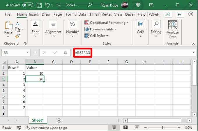
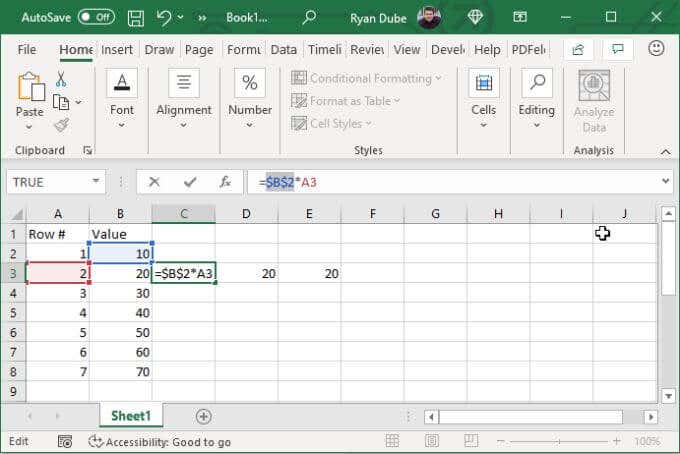
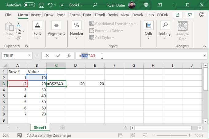
Let’s say your spreadsheet has a “10” in a top row, and you want every row beneath it to multiply that number by the number in the cell to the left. 

To do this, you’d enter a formula that looks like this:

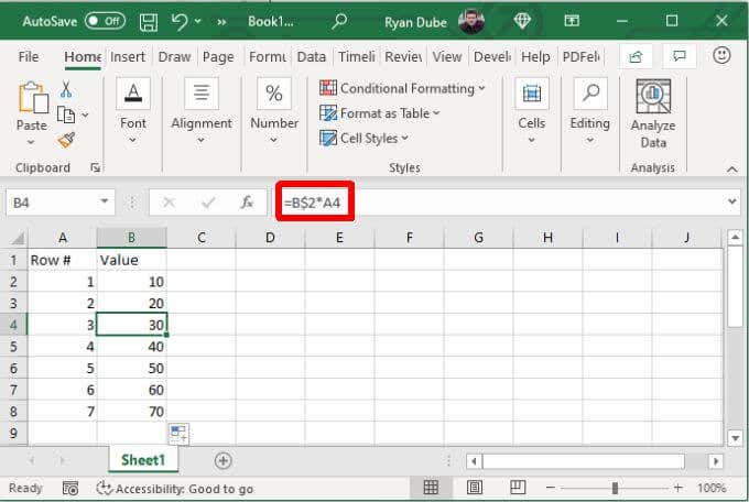
=B$2*A3

This locks the “2” reference so it won’t change the row reference if you drag the cell with this formula down to the cells below it. Since A3 remains “unlocked” both the row and column reference will still change automatically and always reference the cell to the left.

You will notice that this only works because you’re dragging down into cells in the same column. So you don’t have to lock column (B) by placing a dollar sign ($) in front of it.

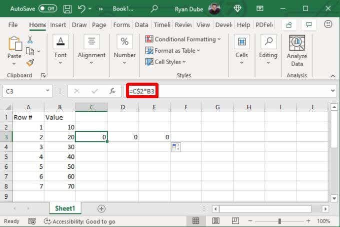
The problem with this is that if you want to use the same formula to the right of the original formula, the “B” reference will change, and the formula will no longer reference B2 as intended.

Let’s take a look at how to use absolute references instead of mixed references to make filling in both directions work properly.

Correctly Using Absolute References in Excel

To use the correct referencing in this formula, you must consider precisely what you’re trying to do.

In this case, we want the following behaviors when filling to the right.

• Always reference the value in cell B2
• Always reference the value in column A
• Shift the reference of the row for column A to the current row of the formula

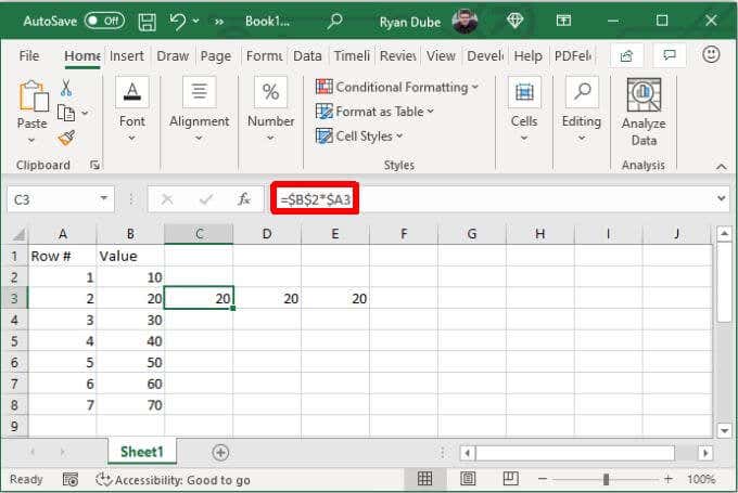
Looking at these behaviors, you now know what you need to “lock” and what you don’t. Both “B” and “2” need to be locked (unchanged). Also, column A needs to be locked.

So your formula in B3 needs to look like this: =$B$2*$A3

Now when you drag this same cell either down or up, the formula works as intended.

Correctly using absolute referencing can get tricky, so it’s essential to take the time to carefully consider how you want Excel to update the formula as you fill columns or rows in either direction.

Cycling Through Reference Types in Excel

You can speed along the process when you’re typing formulas with absolute references by pressing the F4 key, which will make the cell reference absolute.

The cursor can be on either side of the cell reference (or even in the middle of it) when you press F4, and it’ll still convert that single reference to absolute.

If you don’t want absolute (for example, mixed instead), keep tapping F4 until the reference looks the way you want.

If you want to add any kind of referencing to other cells in the formula, just place your cursor there and start cycling through F4 again.

Once you have configured your formula, just press Enter and begin filling your spreadsheet in any direction you like. If you set up your references right, everything should work just as expected.