Alternating the colors of rows and columns in Excel, also known as banding, is one way to make the document easier to read. This practice is helpful when you have documents with lots of data, whether a school or work project. Microsoft Excel doesn’t have a dedicated button to alternate row and column colors, so you’ll have to be creative to achieve the result of banded rows.
An Excel document offers several ways to alternate row and column colors. For example, you can select specific rows and columns and apply a color to each one of them. Although this might sound like a simple solution, manually applying row and column colors would be tedious if your Excel spreadsheet contains thousands of entries. Imagine having to do it to all the documents in a workbook. So, let’s see what you can do to alternate row and column colors in Microsoft Excel quickly.
1. Color Rows and Columns Using Table Style Banding
Using the predefined table styles is a quick way to apply alternate colors to the rows in the Excel document. All you’ll have to do is select your cells and convert them to a table.
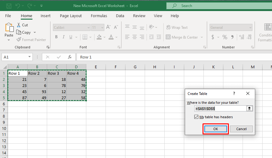
Converting Excel cells and rows into a table is easy. Just select them and press Ctrl + T on your keyboard. This Excel keyboard shortcut will automatically turn your selection into a table, and no data in the cells will be lost. Click OK when prompted.
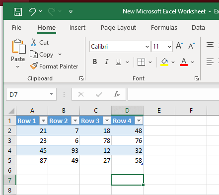
A table made this way will have an automatic row banding applied to it. The odd and even rows of your table will be shaded in different colors, and the banding will continue even when you add or remove rows to your table.
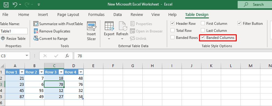
If you want to switch to banded columns instead of rows:
- Select the table or one cell in the table, then go to the Design tab.
- Find the Table Style Options group.
- Tick the Banded Columns box, and untick the Banded Rows.
Remember, you can apply this method to the whole document, but it’s not the best solution for too much data or multiple worksheets. Perhaps it would be smarter to consider using the Conditional Formatting instead.
Change the Table Style
If you don’t like the colors applied to the Excel table with automatic banding (typically, they’re blue and white), you can change them. Here’s how:
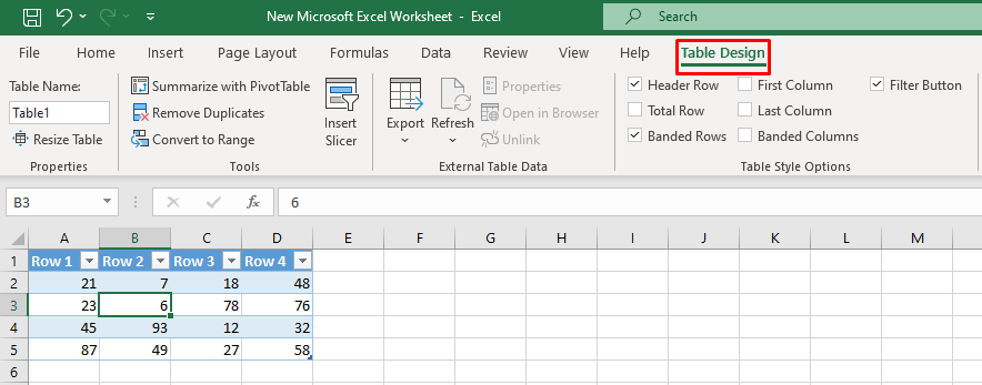
- Click anywhere in your table to select any cell to bring up the Table Design tab in the Excel ribbon.
- Locate the Table Styles group in the Table Design tab.
- Use the arrow buttons on the side of the group to scroll through the styles.
- Select a style you want to apply to your table.
Use the Custom Table Style
If you need to highlight a different number of rows in a different stripe (instead of every other row), you’ll need to create a custom table style.
- Select a cell in your table and go to the Table Design tab.
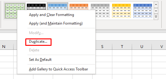
- Right-click on the table style you want to apply and select Duplicate from the menu.
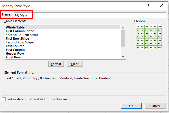
- In the dialog box, enter the name of your custom table style in the Name field.
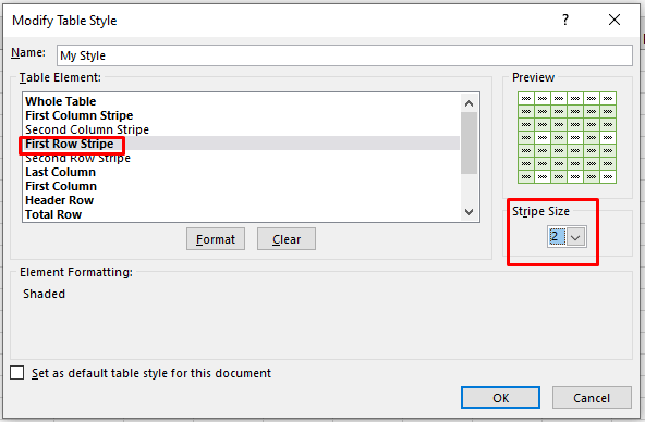
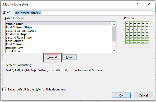
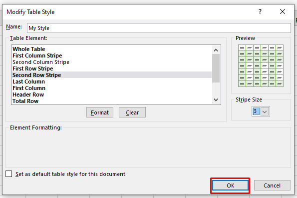
- From the list, select First Row Stripe (First Column Stripe if you want shaded columns) and set the Stripe Size to the value of your choosing. This will depend on how many rows you want colored in the same stripe.
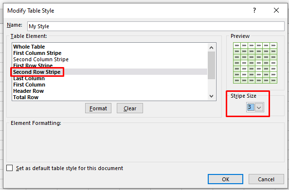
- Select Second Row Stripe (or Second Column Stripe if you want shaded columns) from the list and enter the chosen value.
- To customize your table style further, click the Format button.
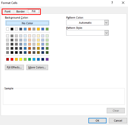
- Select the Font, Border, or Fill tab from the new dialog box to modify your style.
- Click OK, and your table style will be saved.
- Apply this newly created style to your table by selecting it from the Table Style Gallery.
Revert to the Original Range
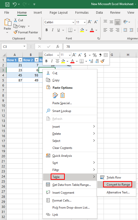
If you don’t want to keep your data within an Excel table and prefer the Excel cells, you can always convert the table back to the usual Excel range. Click anywhere in your table to select a random cell, then right-click. Select Table from the menu, then click Convert to Range from the context menu.
However, when you do this, the automatic banding will stop. Although the rows you selected will remain shaded, no new rows you add will be colored.
Related: Learn to freeze rows and columns in Excel for easier data reference.
2. Alternate Row Colors With Conditional Formatting
Using conditional formatting to color rows in an Excel document is trickier. However, this process will help you be as creative as you want with zebra striping your worksheets. In this section, you’ll learn how to color every other row and add a second color or color the groups of rows. There’s a different formula for different types of shading you want to apply.
Highlight Every Other Row and Column With Conditional Formatting
Highlighting every other row or column with Conditional Formatting will have the same effect as doing it with Table Styles. The difference is that you’ll work directly with Excel cells instead of converting your data to a table and back to the original range. Furthermore, with conditional formatting, the color banding will remain intact even when you add or delete rows and columns.
Follow these steps:
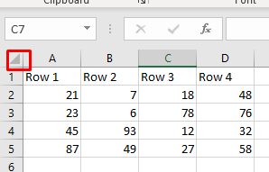
- Select the cells you want to color. You can select all cells to apply the color banding to the worksheet. Simply click the button in the top-left corner of the spreadsheet.
- Go to the Home tab and find the Styles group.
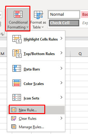
- Click Conditional Formatting and select New Rule… from the drop-down menu.
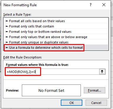
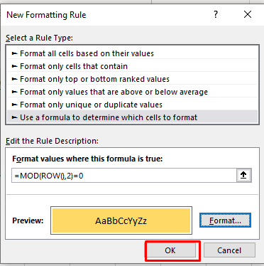
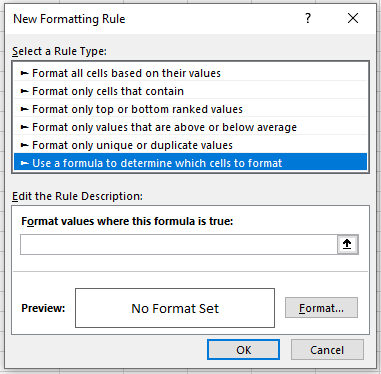
- When the Formatting Rule window opens, select Use formula to determine which cells to format.
- In the Format values box type the following formula: =MOD(ROW(),2)=0
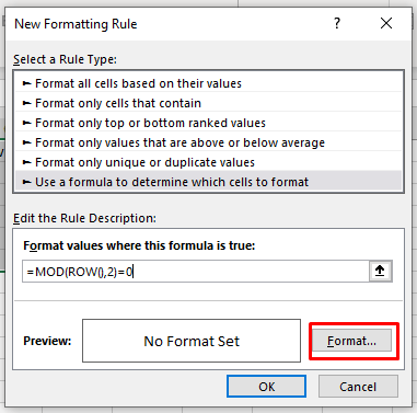
- Select Format.
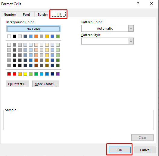
- Modify the background color for your banded rows in the Fill tab.
- When you are happy with the color, click OK.
- Click OK in the New Formatting Rule window to apply the changes.
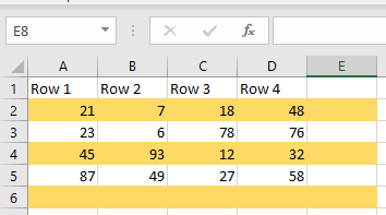
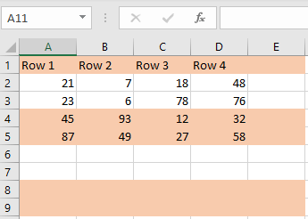
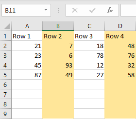
Your Excel document should now look like this:
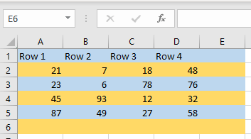
If you want to fill the white rows with different colors, you’ll need to repeat these steps. Create a new rule but this time use this formula: =MOD(ROW(),2)=1
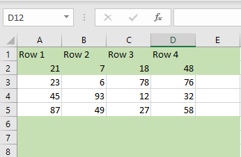
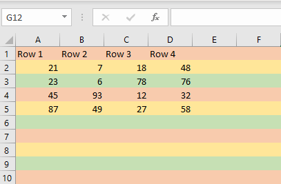
Select a different color, and your Excel document should look similar to this:
As you may have noticed, to color even rows, you’ll use the value 0, and to color odd rows you’ll use the value 1.
Alternate Groups of Rows With Different Colors
Shading groups of rows with Conditional formatting demands a more complex formula. But the steps remain the same.
To highlight the first and every other group you’ll use:
=MOD(ROW()-RowNum,N*2)+1<=N
To highlight the second group and all even groups you’ll use:
=MOD(ROW()-RowNum,N*2)>=N
Note: N is the number of rows in each group, and you get to determine it. This means you should substitute the N in the formula with your chosen number.
Here are some examples:
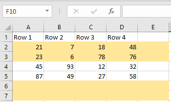
Color every two rows (starting from the first group): =MOD(ROW()-2,4)+1<=2
Color every two rows (starting from the second group): =MOD(ROW()-2,4)>=2
Color every three rows (starting from the second group): =MOD(ROW()-3,6)>=3
Color rows with three different colors (you’ll use three formulas to achieve this): =MOD(ROW()+3-1,3)=1
=MOD(ROW()+3-1,3)=2
=MOD(ROW()+3-1,3)=0
3. Color Alternate Columns with Conditional Formatting
If you want to apply colors to columns instead of rows through conditional formatting, the only thing that’s different is the formula you’d use. All other steps for the Conditional Formatting Rule are the same.
- Select the document or the range of cells that you want to shade.
- In the Home tab, select Conditional Formatting, and go to the New Rule.
- Select Use a formula to determine which cells to format.
- Enter the correct formula.
- Select Format and choose the color from the Fill tab. Click OK when you are satisfied with your choice.
- Click OK in the New Format Rule window to apply the shading to your columns.
Here are some example formulas for coloring the columns in your Excel Document:
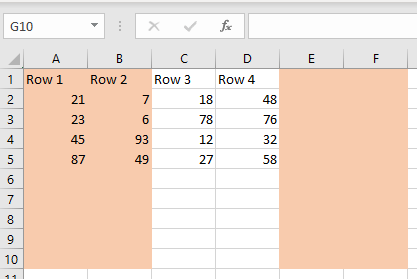
Color every other column: =MOD(COLUMN(),2)=0 or =MOD(COLUMN(),2)=1
Color group of two columns (starting from the first group): =MOD(COLUMN()-1,4)+1<=2
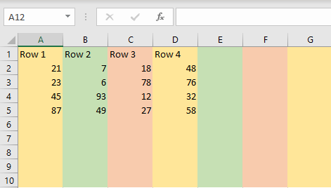
Color Columns with three different colors:
=MOD(COLUMN()+3,3)=1
=MOD(COLUMN()+3,3)=2
=MOD(COLUMN()+3,3)=0
Alternating row and column colors in Microsoft Excel is a valuable skill for anyone working with spreadsheets. It enhances the visual appeal of your data and aids readability, making complex information easier to understand at a glance.
Related Posts
Nicolae is a Jack of all trades technology writer with a focus on hardware, programming languages, and AI image-processing software. Over the last five years, he has ghostwritten numerous tech how-to guides and books on a variety of topics ranging from Linux to C# programming and game development. Nicolae loves everything that has to do with technology and his goal is to share his knowledge and experience with others. Read Nicolae’s Full Bio
