Mathematically, you calculate a range by subtracting the minimum value from the maximum value of a particular dataset. It represents the spread of values within a dataset and is useful for measuring variability – the larger the range, the more spread out and variable your data is.
Luckily, finding the range of a set of data is easy when using Excel functions. Here’s how to do it.
How to Find and Calculate Range in 3 Steps
The easiest way to find the range in Microsoft Excel is by using the MIN and MAX functions. The MIN function calculates the highest value in a set of data, while the MIN function calculates the smallest value.
First, ensure that your data is neatly organized in your worksheet for ease of analysis. Then, you can use the MIN and MAX functions as follows:
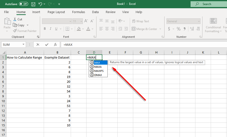
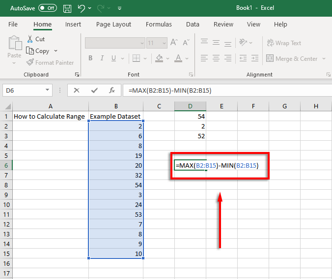
- Select a cell outside of your dataset (in our example D1). In this cell, type =MAX and select =MAX from the drop-down menu.
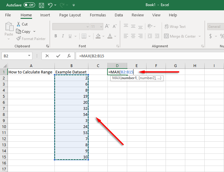
- Select your range of cells by clicking and dragging. Alternatively, you can type the cell range into the cell manually (for example, =MAX(B2:B15). Press Enter to confirm.
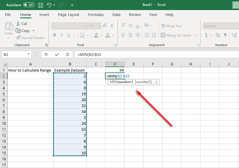
- Select another cell (in our example D2) and type =MIN. Repeat step 2 for this cell.
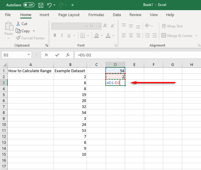
- Now you need to find the difference between these values. To do this, select a cell (in our example, D3) and use the subtract function by typing =(the cell that contains MAX value)-(the cell that contains MIN value). For example, =D1-D2.
It’s possible to calculate the range of values in one shortcut step by combining these functions in one cell. To do so, we’ll use our example where the dataset is contained in cells B2 to B15.
Using these cells, the range function would look like the following:
=MAX(B2:B15)-MIN(B2-B15)
All you have to do is change the cell values to match your data.
How to Find a Conditional Range in Excel
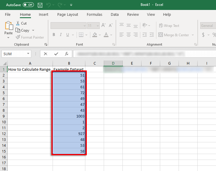
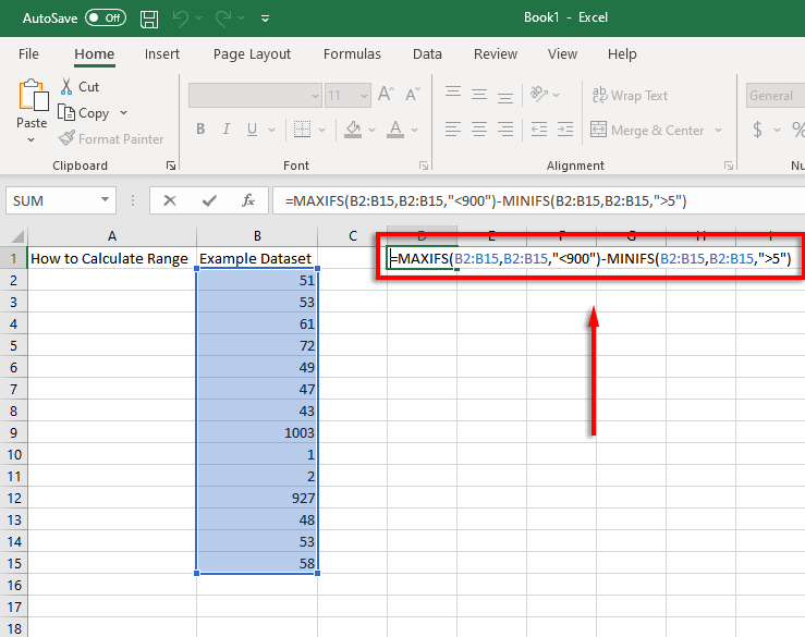
If your set of data has a few outliers, it’s possible to calculate a conditional range that ignores the outliers. For instance, take a look at this example screenshot:
Almost all of the values are between 40 and 80, yet there are two around 1,000 and the two lowest values are close to 1. If you wanted to calculate the range but ignore those values, you would need to ignore values under 5 and over 900. This is where the MAXIFS and MINIFS functions come in.
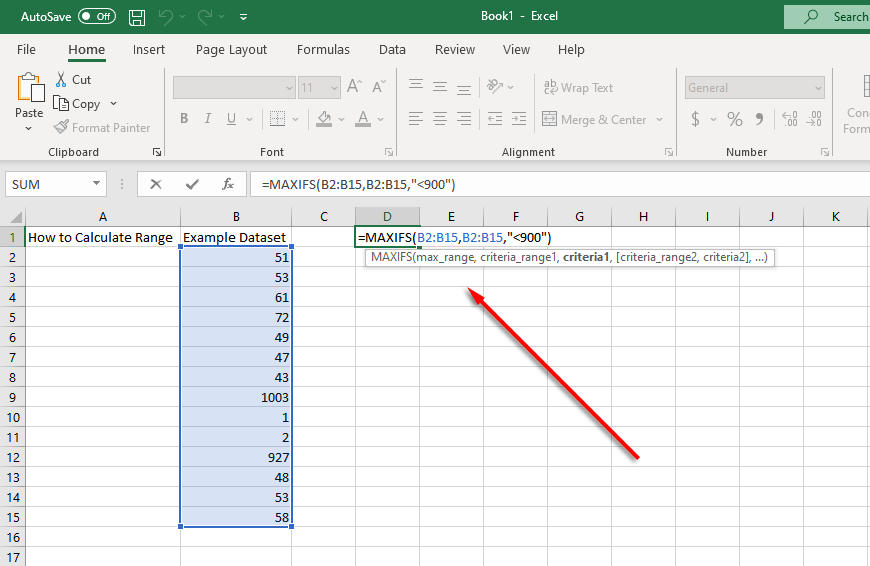
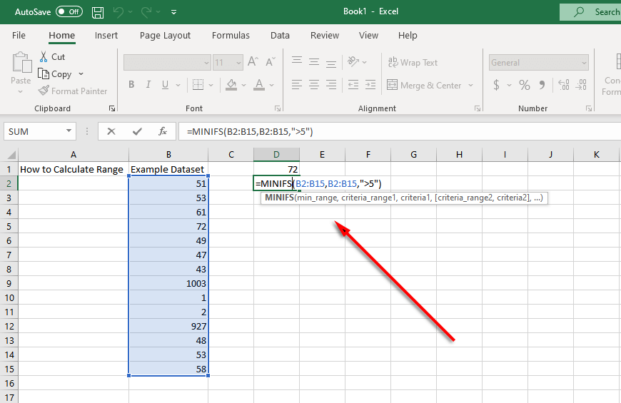
MAXIFS adds a condition that ignores values over a certain number, while MINIFS ignores values lower than a certain number (with each condition separated by a comma).
So, for our example, the MAX function would become:
=MAXIFS(B2:B15,B2:B15,”<900”)
And the MIN function would become:
=MINIFS(B2:B15,B2:B15,”>5”)
In this case, the total Excel formula for calculating the conditional range will be:
=MAXIFS(B2:B15,B2:B15,”<900″)-MINIFS(B2:B15,B2:B15,”>5″)
Note: The MAXIFS and MINIFS functions are only available in Excel 2019 and Microsoft Office 365, so if you’re using an older version, you will need to include the IF function separately. For example: =MAX(B2:B15)-MIN(IF(B2:B15>5,B2:B15)
Data Analysis Has Never Been Easier
Microsoft Excel is a powerful tool for analyzing data. With this tutorial, you can easily calculate the range of any dataset, even if you need to remove outliers.
Related Posts
Jake Harfield is an Australian freelance writer whose passion is finding out how different technologies work. He has written for several online publications, focusing on explaining what he has learned to help others with their tech problems. He’s an avid hiker and birder, and in his spare time you’ll find him in the Aussie bush listening to the birdsong. Read Jake’s Full Bio
