
You’ve got an Excel workbook with thousands of numbers and words. There are bound to be multiples of the same number or word in there. You might need to find them. So we’re going to look at several ways you can find matching values in Excel 365.
We’re going to cover finding the same words or numbers in two different worksheets and in two different columns. We’ll look at using the EXACT, MATCH, and VLOOKUP functions. Some of the methods we’ll use may not work in the web version of Microsoft Excel, but they will all work in the desktop version.
What’s An Excel Function?
If you’ve used functions before, skip ahead.
An Excel function is like a mini app. It applies a series of steps to perform a single task. The most commonly used Excel functions can be found in the Formulas tab. Here we see them categorized by the nature of the function –
- AutoSum
- Recently Used
- Financial
- Logical
- Text
- Date & Time
- Lookup & Reference
- Math & Trig
- More Functions.

The More Functions category contains the categories Statistical, Engineering, Cube, Information, Compatibility, and Web.
The Exact Function
The Exact function’s task is to go through the rows of two columns and find matching values in the Excel cells. Exact means exact. On its own, the Exact function is case sensitive. It won’t see New York and new york as being a match.
In the example below, there are two columns of text – Tickets and Receipts. For only 10 sets of text, we could compare them by looking at them. Imagine if there were 1,000 rows or more though. That’s when you would use the Exact function.
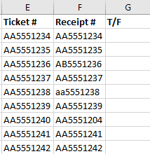
Place the cursor in cell C2. In the formula bar, enter the formula
=EXACT(E2:E10,F2:F10)
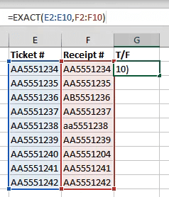
E2:E10 refers to the first column of values and F2:F10 refers to the column right next to it. Once we press Enter, Excel will compare the two values in each row and tell us if it’s a match (True) or not (False). Since we used ranges instead of just two cells, the formula will spill over into the cells below it and evaluate all the other rows.
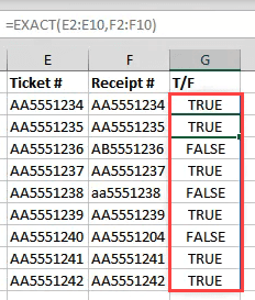
This method is limited though. It will only compare two cells that are on the same row. It won’t compare what’s in A2 with B3 for example. How do we do that? MATCH can help.
The MATCH Function
MATCH can be used to tell us where a match for a specific value is in a range of cells.
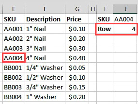
Let’s say we want to find out what row a specific SKU (Stock Keeping Unit) is in, in the example below.
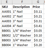
If we want to find what row AA003 is in, we would use the formula:
=MATCH(J1,E2:E9,0)
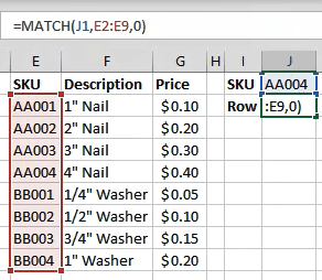
J1 refers to the cell with the value we want to match. E2:E9 refers to the range of values we’re searching through. The zero (0) at the end of the formula tells Excel to look for an exact match. If we were matching numbers, we could use 1 to find something less than our query or 2 to find something greater than our query.
But what if we wanted to find the price of AA003?
The VLOOKUP Function
The V in VLOOKUP stands for vertical. Meaning it can search for a given value in a column. What it can also do is return a value on the same row as the found value.
If you’ve got an Office 365 subscription in the Monthly channel, you can use the newer XLOOKUP. If you only have the semi-annual subscription it will be available to you in July 2020.
Let’s use the same inventory data and try to find the price of something.

Where we were looking for a row before, enter the formula:
=VLOOKUP(J1,E2:G9,3,FALSE)
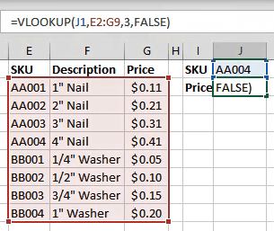
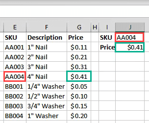
J1 refers to the cell with the value we’re matching. E2:G9 is the range of values we’re working with. But VLOOKUP will only look in the first column of that range for a match. The 3 refers to the 3rd column over from the start of the range.
So when we type a SKU in J1, VLOOKUP will find the match and grab the value from the cell 3 columns over from it. FALSE tells Excel what kind of match we’re looking for. FALSE means it must be an exact match where TRUE would tell it that it has to be a close match.
How Do I Find Matching Values in Two Different Sheets?
Each of the functions above can work across two different sheets to find matching values in Excel. We’re going to use the EXACT function to show you how. This can be done with almost any function. Not just the ones we covered here. There are also other ways to link cells between different sheets and workbooks.
Working on the Holders sheet, we enter the formula
=EXACT(D2:D10,Tickets!E2:E10)
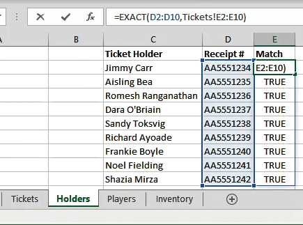
D2:D10 is the range we’ve selected on the Holders sheet. Once we put a comma after that, we can click on the Tickets sheet and drag and select the second range.
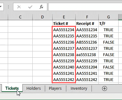
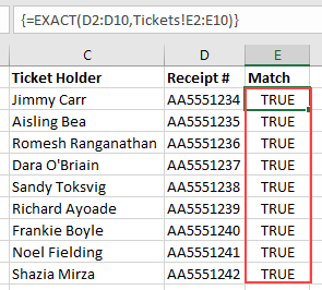
See how it references the sheet and range as Tickets!E2:E10? In this case each row matches, so the results are all True.
How Else Can I Use These Functions?
Once you master these functions for matching and finding things, you can start doing a lot of different things with them. Also take a look at using the INDEX and MATCH functions together to do something similar to VLOOKUP.
Have some cool tips on using Excel functions to find matching values in Excel? Maybe a question about how to do more? Drop us a note in the comments below.