How To Fix a Row In Excel

Dealing with very large Excel spreadsheets isn’t always easy. This is especially true when you have lots of embedded calculations where results in one row depend on data in other rows. Knowing how to fix a row in Excel involves manipulating the sheet in ways where those calculations don’t break.

Other issues that can cause problems when you change cell data is that it’s difficult to see labels in the top row or the left column. 

There are tricks you can use to manipulate large spreadsheets by fixing a row in Excel so you can modify other data without causing any problems.

How To Fix a Row In Excel By Freezing

Need to fix a row in place so that you can still see the header or other columns while you’re editing other areas of the column?

This is very easy. Select the View menu. Then select Freeze Panes from the Window group in the ribbon. Select Freeze Panes from the drop down menu.

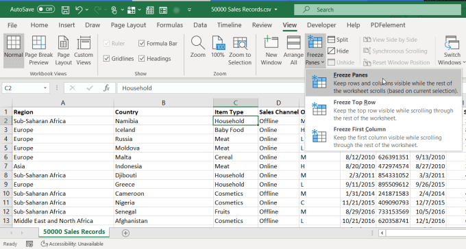
This option fixes both the rows above where your cursor is, as well as the columns to the left of where your cursor is.

If you wanted to only freeze the rows above or the columns to the left, you could use one of the other options.

• Freeze Top Row: Only fix the top row of the sheet in place.
• Freeze First Column: Only fix the left row of the sheet in place.

The “freezing” feature in Excel is very useful, especially for very large sheets where you need to scroll so far to the right or down that the label row or column gets shifted off of the sheet.

Freezing any row or column fixes it in place so you can see it no matter where else you move the cursor in the spreadsheet.

Add a New Row With Fixed Calculations

In a large sheet like this, it can be difficult to add or delete a row and see the result of a calculation update at the bottom of a column or end of a row. And since calculations are usually at the very bottom or the right of a sheet, the result is usually not listed on the sheet when you’re trying to delete or add a row.

If you try to use the freeze option to fix that bottom or right cell, it won’t work. This is because the freeze feature only freezes rows above or to the right of the cursor.

The trick to fix the calculation row or column in place is to use the Excel Split feature.

To do this, place the cursor on the calculation you want to fix in place. Select View from the menu, and then select Split from the Windows group in the ribbon.

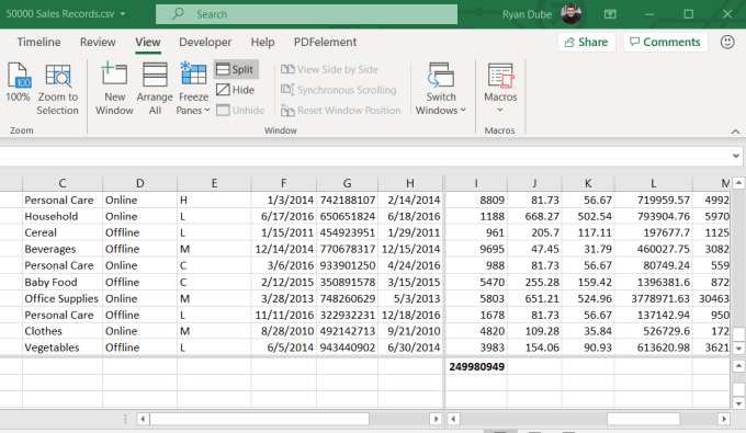
This will fix the calculation at the bottom of the column in place. Now you can right click the gray numbers to the left of any row, and select Delete.

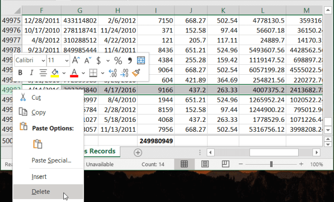
When the row deletes, you can watch the calculation automatically update so that you know it incorporated the change.

This same approach also works if the calculation is at the end of a row. Just place the cursor on the calculation, split the sheet, and delete the column. You’ll see the calculation automatically update.

How To Fix All Row Heights In Excel

While this trick isn’t technically fixing a row in place, it’s a way to format all rows in Excel at once. This will save a lot of time over individually adjusting rows one at a time. This is especially helpful in a massive spreadsheet. 

To adjust the height of all rows in the sheet, select every row. Then, right-click any of the gray numbers to the left of the rows and select Row Height from the menu.

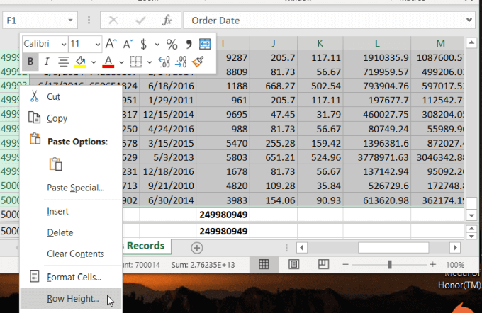
This will open a new window where you can type the row height. Row height is measured in points, and there are 72 points in an inch. Default row height is 12.75, which fits font size of 10 or 12 points. For larger fonts or images, you can type any larger height size that works.

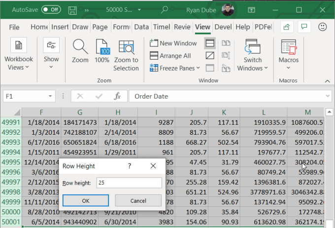
When you select OK, it’ll adjust the height for all of the rows in the sheet that you selected.

Edit Only One Cell In a Row

Another thing people struggle with in a large sheet with a lot of rows is editing or inserting a cell in a single row, without adversely affecting the rest of the sheet.

For example, if you’ve inserted a new data row into the sheet, but there’s an extra data point you want to remove to align it with the rest of the sheet, you’ll need to delete the single cell in that row.

To do this, select and right-click that single cell. Select Delete from the drop-down menu. Since the single cell is in the middle of the spreadsheet and surrounded by data, Excel will display a special Delete window.

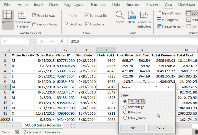
This window lets you shift all of the other data cells back into the right spots to align with the rest of the sheet.

• Shift cells left: All cells to the right of the deleted cell will shift left.
• Shift cells up: All cells under the deleted cell will shift up.
• Entire row: This will delete the entire row that contains the selected cell.
• Entire column: This will delete the entire column that contains the selected cell.

All of these Excel tricks let you fix a row (or a column) in Excel while maintaining calculations or positions of the rest of the data in the sheet.