How To Merge Cells, Columns & Rows In Excel

When working with data in Excel, it’s common to merge cells, columns, and rows to combine numbers or text.

There are different reasons you may need to merge information in Excel. Sometimes it’s to improve formatting. Other times it’s to bring information from multiple cells into a single cell.

Whatever the reason, you can use the following methods to combine information in Excel in any way you need to.

How to Merge Cells in Excel

One of the most common reasons to merge multiple cells is when you’re creating a title row in your Excel spreadsheet.

1. You can create the title text inside any of the cells that you’d like to merge. Format the text to appear however you’d like, including font size, style, and vertical alignment or height.

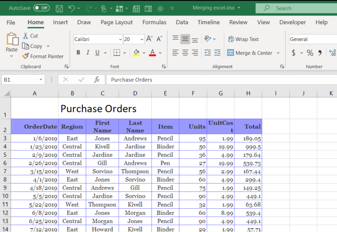
2. Next, you’ll want to make sure the text is aligned perfectly over the width of your data table. To do this, select all of the cells that you want to merge and center.

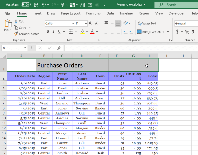
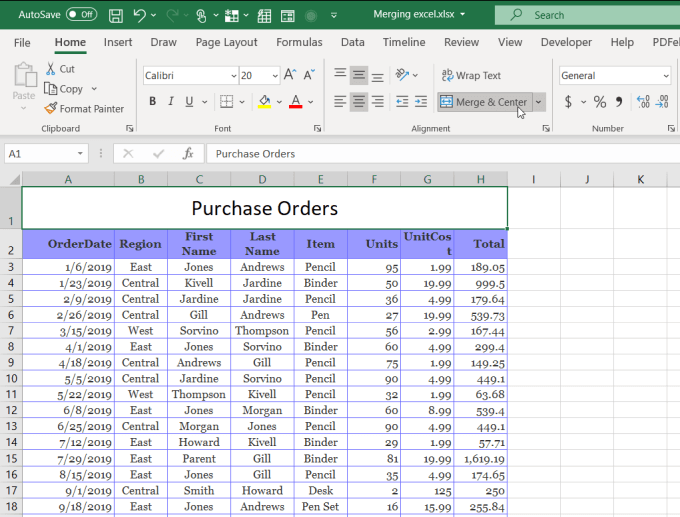
3. With all cells you want to merge selected, on the Home menu select Merge & Center. This will combine all selected cells into one single cell, and center the text or data in that cell. 

You can do the same for cells vertically as well. For example, if you want to have the name of the month centered vertically on the right side of all rows for that month, you can do this using Merge Cells.

To do this:

1. Type the name of the month in the first cell.

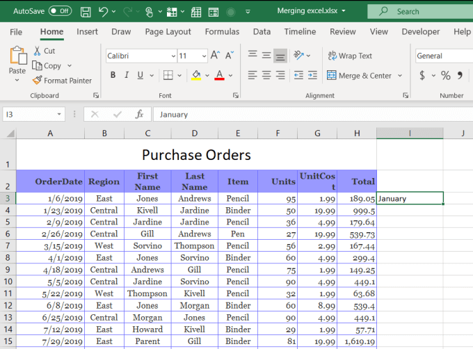
2. Next, select all of the cells that are relevant. So in this case, January would include the first and second cells.

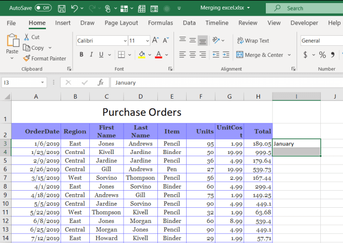
3. Now, with those cells selected, in the Home menu select the dropdown arrow next to Merge & Center. Select Merge Cells from the dropdown menu.

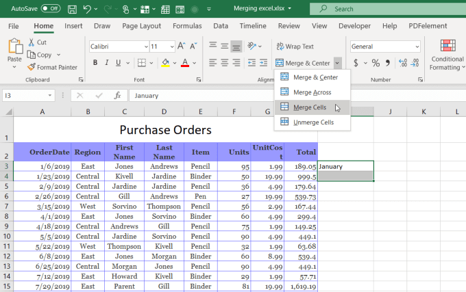
This will merge those cells in Excel into one and place the text at the bottom of the cell by default. The reason you don’t want to use Merge & Center in this case is because that will center the text horizontally in the column. 

In this case, you’d probably prefer to center the text vertically so it’s in the center of all of the cells it applies to. To do this just select the newly merged cell, and select the vertical center alignment icon in the Home menu in the Alignment ribbon group.

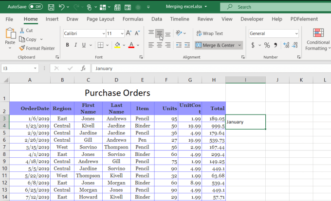
This aligns the text vertically with all of the relevant cells so that everything lines up perfectly.

How to Merge Columns in Excel

In Excel, you aren’t limited to merging individual cells. You can also merge entire columns of data.

For example, in this example spreadsheet, you may want to combine the First Name and the Last Name of the sales associate into another column for their full name.

In this spreadsheet, if you select all of the data in the two columns and try to merge the cells using Merge & Center, you’ll see an error message that you’ll lose the data in all of the cells except the first cell in the range. 

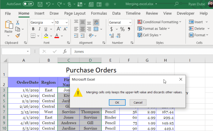
This isn’t useful at all.

There are a couple of quick ways you can combine all data from two columns without losing anything. 

Merge Columns Using Notepad

One easy way to combine data from the two columns into one is copying all of the data from the two columns into notepad. Notepad’s search and replace feature is an effective way to quickly format the two pieces of data into one.

1. Copy all of the cells from the two columns you want to merge and paste them into Notepad. Go to the bottom of the list and press Tab on your keyboard. Highlight that tab space and copy it using Ctrl-C. You’re going to need this later. Then highlight all of the text.

2. Select the Edit menu, and select Replace.

3. In the Find what field, press Ctrl-V to paste the Tab character. In the Replace with field, press the spacebar. This will replace all tabs in the document with a single space.

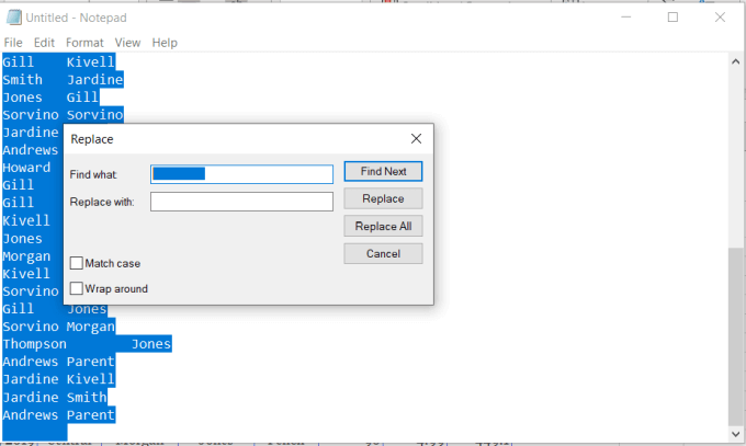
4. Now select Replace All, and all of the text in the Notepad document should appear normal, with the first name and last name separated by just a single space.

5. Highlight all text in the document and press Ctrl-C to copy. Go back to your sheet and paste using Ctrl-V into the top of the first column you originally copied from.

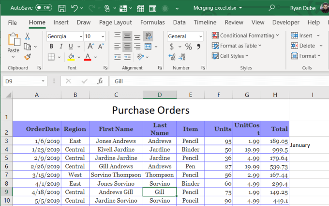
6. Finally, just rename the first column and delete the second one. Now your spreadsheet has the two columns merged into one.

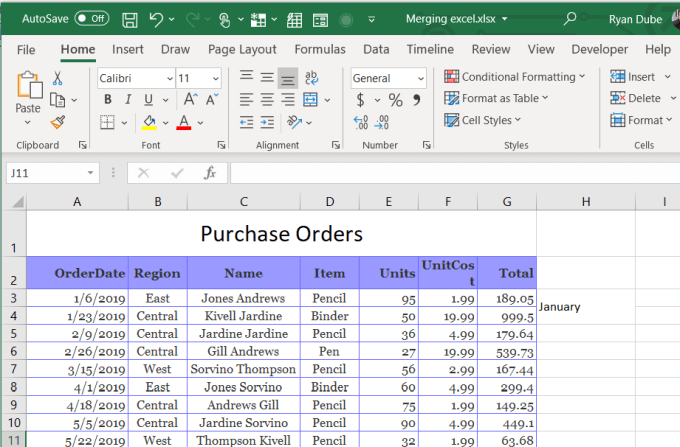
This isn’t the most sophisticated way to merge columns in Excel, but it works and it’s easy.

Merge Columns In Excel Using Concatenate

If you do want to get a little more sophisticated and save a few steps in the process, you could use the CONCATENATE function in Excel. This function works just like the Concatenate function in Google Sheets.

This function combines text from multiple cells into one. You could even use it to merge as many columns as you want, not just two.

1. To do this, right click the column to the right of the two you want to merge and select Insert. This will insert a new, blank column. 

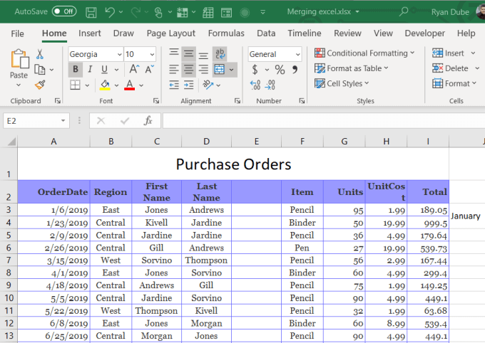
2. In the first blank cell at the top of this new blank column, type =CONCATENATE(C3,” “,D3). Replace C3 and D3 with whatever cells contain your data. The “ “ in the middle adds a space between the text from the two cells. When you press enter, you’ll see the data from the two cells put together with a space between them.

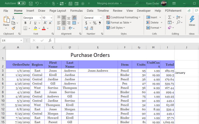
3. Finally, to copy this function down the entire column and merge data from both of the columns, hold down Shift on your keyboard and hover your mouse over the lower right corner of the first cell until the mouse icon changes to two horizontal lines. Then double-left click the mouse.

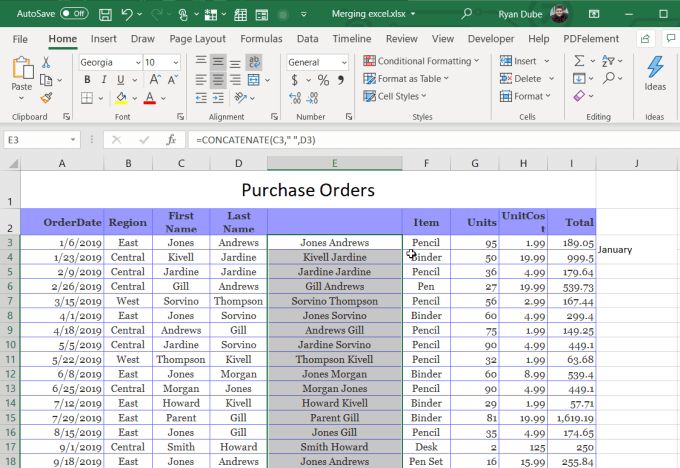
This is an automated fill feature in Excel. It’ll fill the formula to the bottom of that column as far as there’s data in the column to the left. Now you can see the entire column has data from the first two columns merged together.

However, in order to delete the first two columns, you’ll need to copy the entire new column and repaste it as values only.

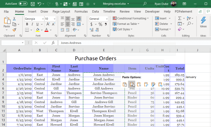
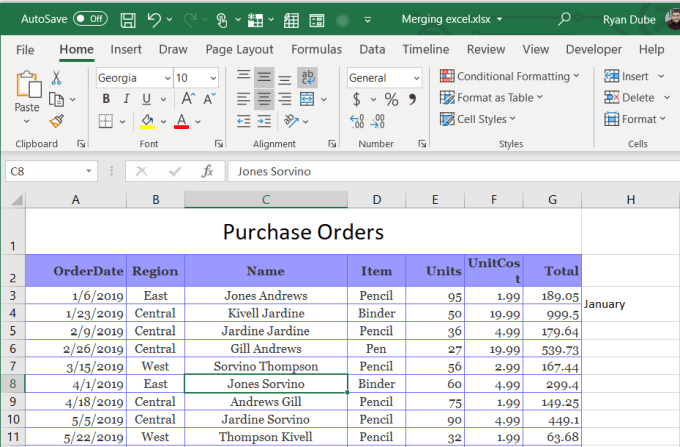
Once you do this, you can delete the two old columns and your spreadsheet is now finished, with the two columns merged into one.

How to Merge Rows in Excel

There is no quick and easy trick or feature to merge rows in Excel. You’ll need to use the same CONCATENATE function as you did for merging columns.

However the technique is a little different. It isn’t very common for people to combine data from different rows into a new row, but the need may arise occasionally.

Merge Rows Using Concatenate

For example, in the sample spreadsheet we’ve been using, what if you wanted to combine all of the team member names from a single month into a new row on a different page? To do this, you’d need to concatenate the names and separate them using a character like a comma.

1. Place the cursor where you want to place the data from multiple rows. For example you might place the cursor in a new sheet. Then type =CONCATENATE(Sheet1!C3,”,”,Sheet1!C4). Replace C3 and C4 by selecting the actual cells in the other sheet that you wanted to concatenate.

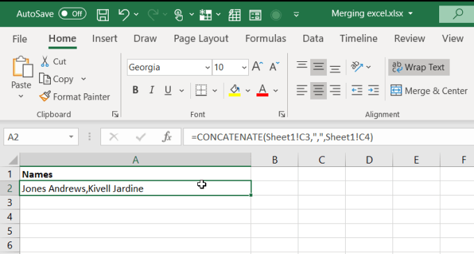
2. When you press Enter, you’ll see the concatenated data appear in the new row, separated by commas. To merge more rows, just copy and paste the first cell into the second new row, and edit the formula to include the rows from the original sheet that you want to merge.

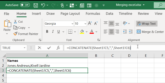
You can continue this process until you’ve merged all of the rows from the original sheet that you want to. Remember, you can freeze the top row in Excel if you need to so that you can still see the header while you’re working on the data.

Merge Rows In Excel Using Merge & Center

Of course the Merge & Center does work for multiple rows that hold the same data. For example in this spreadsheet, both February entries are from the “Central” region. Instead of repeating this twice, you could merge these two rows into one.

1. Highlight both rows that you want to merge.

2. In the Home menu, select Merge & Center from the ribbon.

As you can see, this combines the two rows containing the same data into a single row containing one of those duplicates.

This is a smart way to clean up your spreadsheets and reduce duplicates throughout the data set.

These are a few of the quickest tips to merge cells, columns, and rows in Excel. Do you know any others? Share them in the comments section below!