If you’ve ever considered taking out a mortgage or any other loan, knowing how to use the PMT function in Excel can give you some insight into what your payments are going to look like.
PMT stands for “Payment”. This is once you provide all of the required inputs into the function, it will return the periodic payment you’ll need to make.
Understanding how the PMT function works in Excel can help you measure how long it’ll take to pay off a loan if you pay a certain amount, or depending how the interest rate changes.
How The PMT Function in Excel Works
The PMT function is much simpler than other Excel functions, like Index or Vlookup. But that doesn’t make it any less useful.
To get the periodic payment on a loan, you need to provide the PMT function with the following inputs.
- rate: The loan interest rate.
- nper: Total number of payments made over the entire period of the loan.
- pv: The starting balance of the loan (present value).
- fv: The cash you have left after the loan is paid off (future value). This is optional and defaults to 0.
- type: Whether payments are due at the beginning of each pay period (1) or the end (0). This is also optional.
An easy way to understand how you can use this function is to start with a simple example.
Let’s say you’re thinking of taking out a personal loan of $10,000 from your bank. You know you want to pay it off in 4 years (48 months), but you aren’t sure what interest rate you’ll get when the bank runs your credit.
To estimate what your payment will be for different interest rates, you can use the PMT function in Excel.
Set up the spreadsheet with the known, fixed values at the top. In this case that’s the loan amount and the number of payments. Create one column of all possible interest rates, and an empty column for the payment amounts.
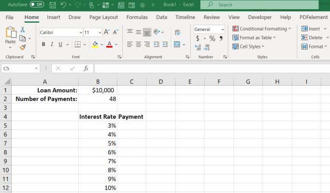
Now, in the first cell for Payment, type the PMT function.
=PMT(B5,B2,B1)
Where B5 is the cell with interest rate, B2 is the cell with the number of payments, and B1 is the cell with the loan amount (present value). Use the “$” symbol for B1 and B2 as shown below to keep those cells constant when you fill the column in the next step.
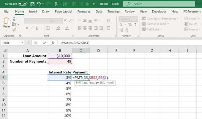
Press Enter and you’ll see the payment amount for that interest rate.
Hold down the Shift key and place the cursor over the lower right corner of the first cell with the payment amount until the cursor changes to two horizontal lines. Double-click and the rest of the column will fill with payments for the other interest rates.
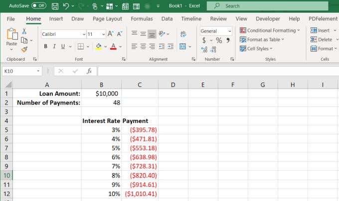
What these results show you is exactly what payment you can expect for this loan, depending what interest rate the bank offers.
What’s useful about using Excel for this is you can also change the cells with the total loan amount or the number of payments and observe how this changes the periodic payment amount of the loan.
Other PMT Function Examples In Excel
Let’s take a look at a couple, slightly more complicated examples.
Imagine you’ve won a large award, and the organization that will give you the award has given you the choice to accept the award in a lump sum or an annuity. You can receive $1,000,000 as a 5% annuity over 10 years, or $750,000 in a lump sum today. Which is the better option in the long run?
The PMT function in Excel can help. In the case of the annuity, you’ll want to know what the annual payment comes to.
To do this, use the same approach as the last example, but this time the known values are:
- future value: $1,000,000
- rate: 5%
- number of payments: 10 (one annual payment over ten years)
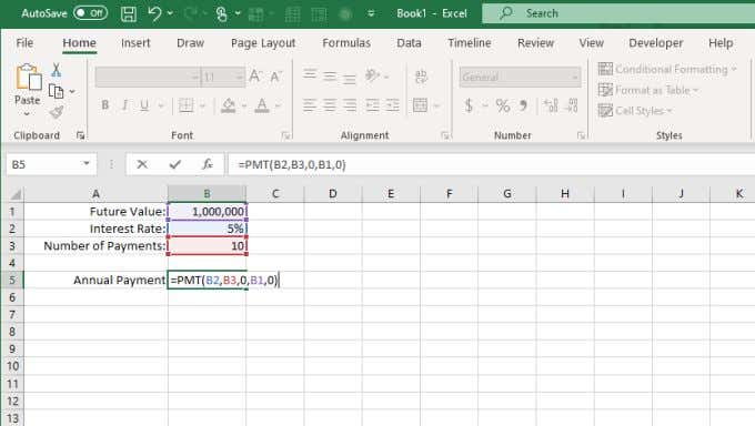
Type the function:
=PMT(B2,B3,0,B1,0)
The zero at the end means the payments will be made at the end of each period (year).
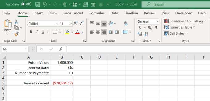
Press Enter, and you’ll see that the annual payment comes to $79,504.57.
Next, let’s look at how much money you would have in 10 years if you take the $750,000 today and put it into an investment that only earns a modest 3% interest rate.
Determining the future value of a lump sum requires a different Excel formula called FV (future value).
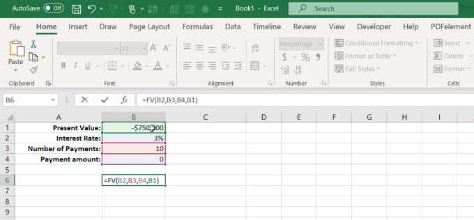
This formula requires:
- Interest rate: 3%
- Number of payments: 10 (years)
- Payments made: 0 (no amount withdrawn)
- Present value: -$750,000 (amount deposited)
This formula is: =FV(B2,B3,B4,B1)
Press Enter and you’ll see that if you invested the entire $750,000 today and only earn 3%, you’d end up with $7,937.28 more in 10 years.
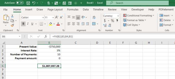
This means taking the lump sum today and investing it yourself is smarter, because you can likely earn much more than just 3% if you invest wisely.
The PMT Function In Excel Is Useful
Whether you’re applying for a home loan, a car loan, or considering lending money out to a family member, the PMT function in Excel can help you figure out the right loan terms for your situation.
So the next time you’re considering walking into a bank or a car dealership, first sit down with Excel and do your homework. Understanding the impact of interest rates and payments will put you at a much better advantage than walking in cold and having to take someone else’s word for it.
If you use Excel a lot, you’ll want to take a look at our tips and tricks for Excel. And if you know of any other cool uses for the PMT function, share them in the comments section below.
