
Have you ever had a large spreadsheet with data in Excel and need an easy way to filter and extract specific information from it? If you learn how to use VLOOKUP in Excel, you can do this lookup with just a single, powerful Excel function.
The VLOOKUP function in Excel scares a lot of people because it has a lot of parameters and there are multiple ways to use it. In this article you’ll learn all of the ways you can use VLOOKUP in Excel and why the function is so powerful.
VLOOKUP Parameters In Excel
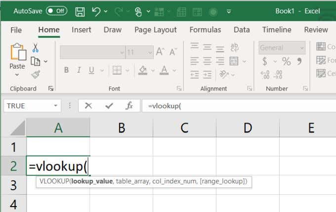
When you start typing =VLOOKUP( into any cell in Excel, you’ll see a pop-up showing all of the available function parameters.
Let’s examine each of these parameters and what they mean.
- lookup_value: The value you’re looking for from the spreadsheet
- table_array: The range of cells in the sheet you want to search through
- col_index_num: The column where you want to pull your result from
- [range_lookup]: Match mode (TRUE = approximate, FALSE = exact)
These four parameters let you do a lot of different, useful searches for data inside of very large datasets.
A Simple VLOOKUP Excel Example
VLOOKUP isn’t one of the basic Excel functions you might have learned, so let’s look at a simple example to get started.
For the following example, we’ll use a large spreadsheet of SAT scores for schools in the United States. This spreadsheet contains over 450 schools along with individual SAT scores for reading, math, and writing. Feel free to download to follow along. There is an external connection that pulls the data, so you’ll get a warning when opening the file, but it’s safe.
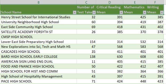
It would be very time consuming to search through such a large dataset to find the school that you’re interested in.
Instead, you can create a simple form in the blank cells on the side of the table. To conduct this search, just make one field for School, and three additional fields for reading, math, and writing scores.
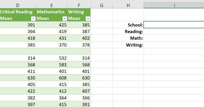
Next, you’ll need to use the VLOOKUP function in Excel to make these three fields work. In the Reading field, create the VLOOKUP function as follows:
- Type =VLOOKUP(
- Select the School field, which in this example is I2. Type a comma.
- Select the entire range of cells that contain the data you want to look up. Type a comma.
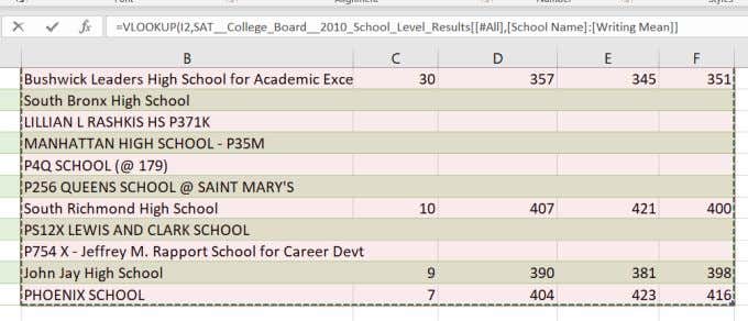
When you select the range, you can start from the column you’re using to look up (in this case the school name column), and then select all of the other columns and rows that contain the data.
Note: The VLOOKUP function in Excel can only search through cells to the right of the search column. In this example, the school name column needs to be to the left of the data you’re looking up.
- Next, to retrieve the Reading score, you’ll need to select the 3rd column from the leftmost selected column. So, type a 3 and then type another comma.
- Finally, type FALSE for an exact match, and close the function with a ).
Your final VLOOKUP function should look something like this:
=VLOOKUP(I2,B2:G461,3,FALSE)
When you first press Enter and finish the function, you’ll notice the Reading field will contain an #N/A.
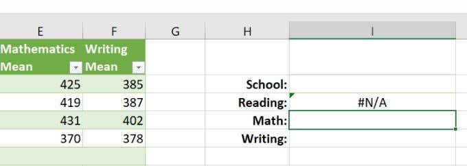
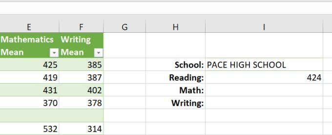
This is because the School field is blank and there is nothing for the VLOOKUP function to find. However, if you enter the name of any high school you want to look up, you’ll see the correct results from that row for the Reading score.
How To Deal With VLOOKUP Being Case- Sensitive
You may notice that if you don’t type the name of the school in the same case as how it’s listed in the dataset, you will not see any results.
This is because the VLOOKUP function is case sensitive. This can be annoying, especially for a very large dataset where the column you’re searching through is inconsistent with how things are capitalized.
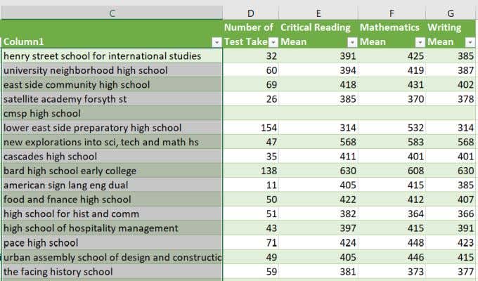
To get around this, you can force what you’re searching for to switch to lowercase before looking up the results. To do this, create a new column next to the column you’re searching. Type the function:
=TRIM(LOWER(B2))
This will lowercase the school name and remove any extraneous characters (spaces) that might be on the left or right side of the name.
Hold down the Shift key and place the mouse cursor over the lower right corner of the first cell until it changes to two horizontal lines. Double click the mouse to autofill the entire column.
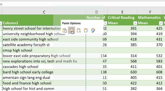
Finally, since VLOOKUP will try to use the formula rather than the text in these cells, you need to convert them all to values only. To do this, copy the entire column, right click in the first cell, and paste values only.
Now that all of your data is cleaned up in this new column, slightly modify your VLOOKUP function in Excel to use this new column instead of the previous one by starting the lookup range at C2 instead of B2.
=VLOOKUP(I2,C2:G461,3,FALSE)
Now you’ll notice that if you always type your search in lower case, you’ll always get a good search result.
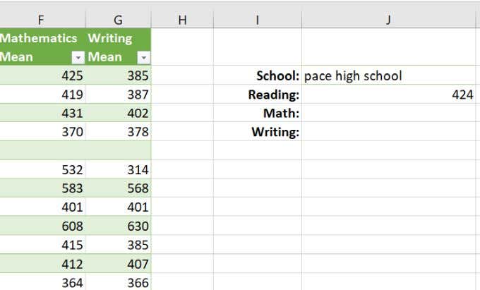
This is a handy Excel tip to overcome the fact that VLOOKUP is case sensitive.
VLOOKUP Approximate Match
While the exact match LOOKUP example described in the first section of this article is pretty straightforward, the approximate match is a little more complex.
The approximate match is best used to search through number ranges. To do this correctly the search range needs to be properly sorted. The best example of this is a VLOOKUP function to search for a letter grade that corresponds to a number grade.
If a teacher has a long list of student homework grades from throughout the year with a final averaged column, it would be nice to have the letter grade corresponding to that final grade come up automatically.
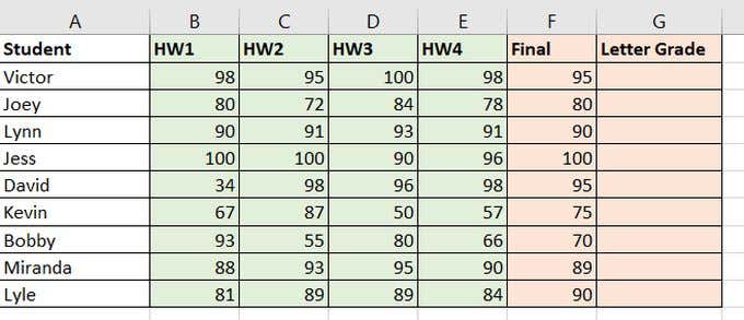
This is possible with the VLOOKUP function. All that’s required is a lookup table off to the right that contains the appropriate letter grade for each numerical score range.
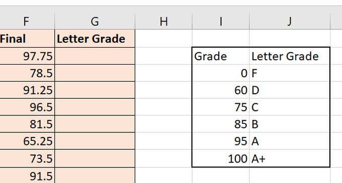
Now, using the VLOOKUP function and an approximate match, you can find the proper letter grade corresponding to the correct numeric range.
In this VLOOKUP function:
- lookup_value: F2, the final averaged grade
- table_array: I2:J8, The letter grade lookup range
- index_column: 2, the second column in the lookup table
- [range_lookup]: TRUE, approximate match
Once you finish the VLOOKUP function in G2 and press Enter, you can fill in the rest of the cells using the same approach described in the last section. You’ll see all of the letter grades properly filled in.
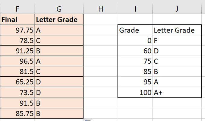
Note that the VLOOKUP function in Excel searches from the bottom end of the grade range with the assigned letter score to the top of the range of the next letter score.
So, “C” needs to be the letter assigned to the lower range (75), and B is assigned to the bottom (minimum) of its own letter range. VLOOKUP will “find” the result for 60 (D) as the closest approximate value for anything between 60 to 75.
VLOOKUP in Excel is a very powerful function that has been available for a long time. It is also useful for finding matching values anywhere in an Excel workbook.
Keep in mind, however, that Microsoft users who have a monthly Office 365 subscription now have access to a newer XLOOKUP function. This function has more parameters and additional flexibility. Users with a semi-annual subscription will need to wait for the update to roll out in July 2020.