There are a surprising number of ways you can make use of a random number generator in Excel. But before you do, it’s important to understand the function of a random number generator and how you can use it for different applications.
Once you learn how to use the random number functions, you can do things like generating dummy sample data to test calculations, choosing the order of players for a game, picking winners for a contest, and many other things.
Random Number Generator Functions in Excel
The two functions in Excel that work to create random numbers include RAND, RANDBETWEEN, and RANDARRAY.
- RAND: Returns a random number between 0 and 1. This is usually a decimal like 0.358432.
- RANDBETWEEN: Returns a random number between two numbers you provide. In other words, if you want a random number between 1 and 100, this function will return an integer value inside that range.
- RANDARRAY: Returns any number of random integers or decimals, between any minimum or maximum numbers, and across any range of rows and columns you want.
Whenever you open a spreadsheet or refresh calculations, both of these functions will generate a new random value. Unfortunately, any change to the spreadsheet triggers an update of these values.
Also, keep in mind that both of these random number functions can generate duplicate values when you use them in multiple cells. It’s more likely that RANDBETWEEN will generate duplicates because RAND generates decimals and there are many more possible numbers.
How to Use the RAND Function
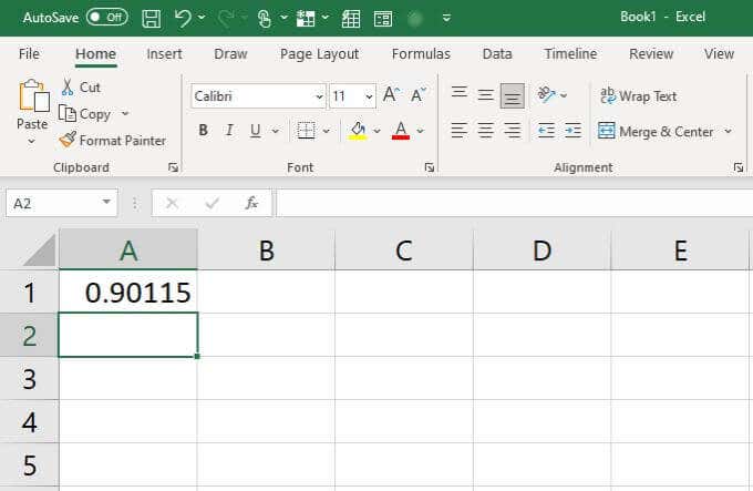
The RAND function is very straightforward to use because there are no arguments at all. Just type “=RAND()” into a cell and press Enter.
This will immediately generate a decimal between 0 and 1.
When to Use the RAND Function
How can such a simple function be useful? Here are a few practical ideas for using the RAND function.
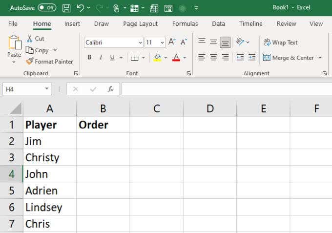
Let’s say you have a list of names of friends playing a board game and you want to quickly sort out the order of play. The RAND function is perfect for this.
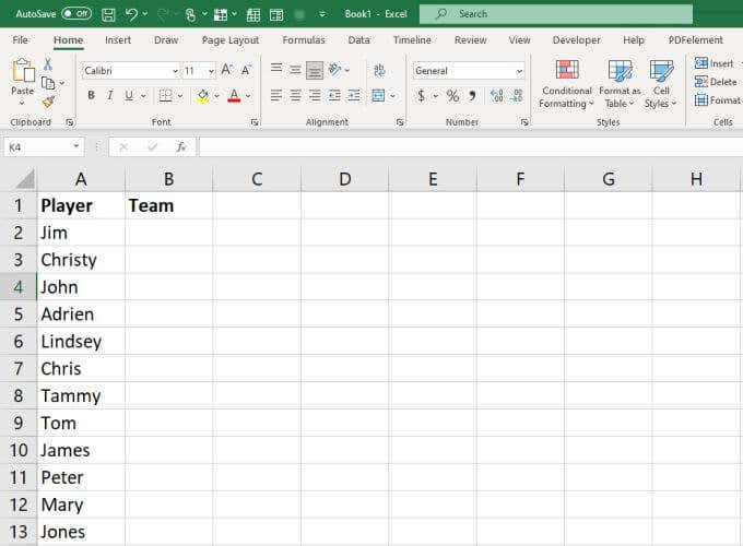
Just list all of the names of your friends in the first column.
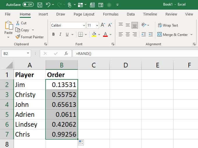
Use the RAND() function to generate random decimals in the next column.
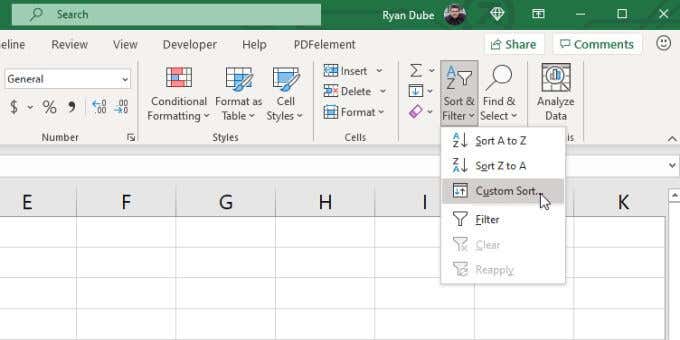
Finally, select both columns, select Home from the menu, select Sort & Filter from the ribbon, and then select Custom Sort.
In the Sort window, choose the column with the random numbers to sort, and order them from Largest to Smallest. Select OK.
This will reorder your list according to the random numbers that were generated. Along with those, it’ll also resort the names into the new order for gameplay.
You can use RAND similarly in any case where you want to randomize a value in a calculation, a list of text values, or anything else stored in your spreadsheet.
How to Use the RANDBETWEEN Function
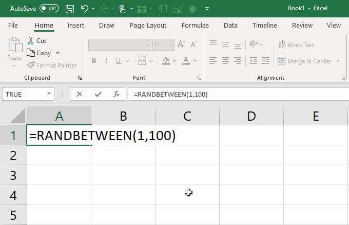
The RANDBETWEEN function is almost as simple as the RAND function to use. Just type “RANDBETWEEN([min],[max]”, replacing min and max with the lowest and highest numbers of the range you want numbers for.
When you press Enter, that cell will contain a random number between that low or high value.
When to Use the RANDBETWEEN Function
The RANDBETWEEN random number generator function is even more useful than the RAND function. This is because it lets you contain the returned random numbers within a range. It also returns integers instead of decimals.
This gives you some very creative ways to use this function to apply random assignments when you want to be fair, or assigning fixed numbers to people or things without showing any bias.
Let’s look at an example. Let’s say you have a list of 12 people and you want to split them into two teams of 6 each without the embarrassment that comes from letting people “pick” their favorite people for each team.
First, create a spreadsheet with all of the players’ names.
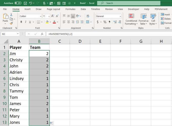
Add the following function to the next column, next to each player name. Then press Enter.
=RANDBETWEEN(1,2)
You can enter this into the first cell and then fill the rest below it. This will automatically assign each player to team 1 or team 2.
If you find that the distribution between the two teams isn’t even, just reenter the function in the first cell and press Enter. This will update all cells again. Repeat until the split between the two teams is even.
How to Use the RANDARRAY Function
The RANDARRAY function is available in Excel 365 only. If you have this version of Excel, this is a very powerful random generator function in Excel that you can use for a wide range of purposes.
Using it is very simple, with lots of optional settings. Just type the following into any cell:
=RANDARRAY ([rows], [columns], [min], [max], [integer])
The parameters are as follows:
- rows: Number of rows to generate random numbers
- columns: Number of columns to generate random numbers
- min: Minimum limit for the numbers
- max: Maximum limit for the numbers
- integer: Whether you want decimals or integers (TRUE or FALSE)
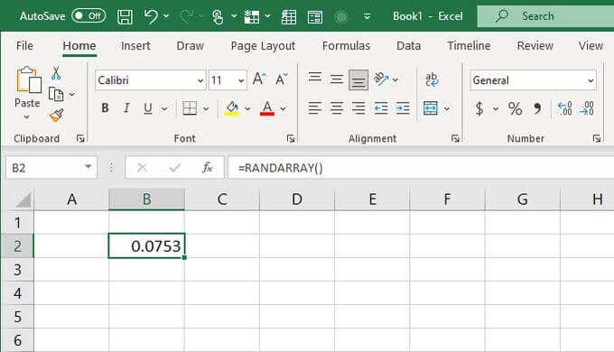
If you just use the RANDARRAY function alone and don’t use any of the optional parameters, it’ll work just like the RAND function.
Just remember that the RANDARRAY function is very flexible and will only fill in as many rows and columns as you specify, in the exact way that you specify. Default is always decimals, and only 1 row and 1 column.
When to Use the RANDARRAY Function
The RANDARRAY function is best used when you need an entire collection of random numbers, including multiple columns and multiple rows.
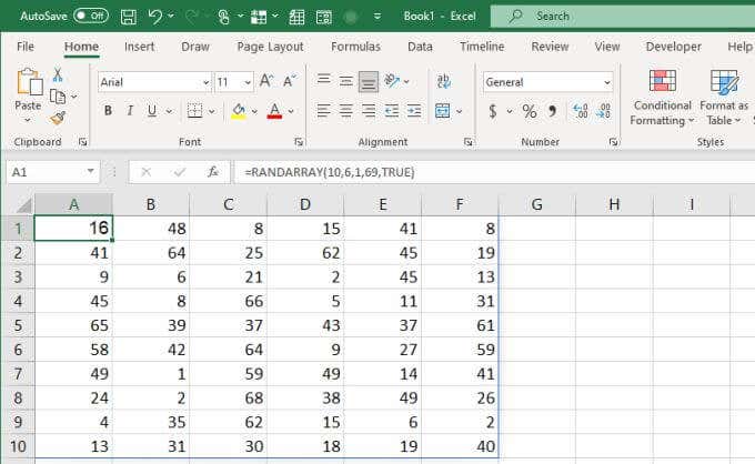
For example, if you’re simulating something like a random list of lottery number choices, you can quickly create a list of rows that contain 6 columns (for the 6 lottery balls). Set the limit to 69 and let Excel guess your 10 lottery picks for you with the following function:
=RANDARRAY(10,6,1,69,TRUE)
Place this into the first cell of your spreadsheet and press Enter.
You’ll see a table generated that includes 10 rows and 6 columns.
This function could be a great solution in science or statistical research if you need a large random dataset and don’t want to build it all manually.
Choosing the Right Random Number Generator in Excel
Whichever of the three Excel functions you use depends mostly on what results you’re looking for. If you don’t really care what the number is, RAND will do just fine. If you want to limit the range of numbers generated, then go with RANDBETWEEN. And if you’re looking for a much larger dataset with an entire table of numbers, that’s when RANDARRAY is the best option for you.
Related Posts
Ryan has been writing how-to and other technology-based articles online since 2007. He has a BSc degree in Electrical Engineering and he’s worked 13 years in automation engineering, 5 years in IT, and now is an Apps Engineer. Read Ryan’s Full Bio


