How to Fix #VALUE! Error in Microsoft Excel

If you’re often working with formulas in Microsoft Excel, you’ve probably encountered the #VALUE error. This error can be really annoying because it’s very generic. For example, adding a text value to the numbers formula might trigger this error. That’s because when you add or subtract, Excel expects you to use only numbers.

The easiest way to deal with the #VALUE error would be to always make sure there are no typos in your formulas, and that you’re always using the correct data. But this might not always be possible so in this article we will help you learn several methods that you can use to deal with the #VALUE error in Microsoft Excel.

Also, check out our favorite Excel tips and tricks to boost your productivity with fewer headaches.

What’s Causing the #VALUE Error

There are several reasons why the #VALUE error might happen when you’re using a formula in Excel. Here are some:

1. Unexpected Data Type. Let’s say you’re using a formula that works with a specific data type, but a cell or several cells in your worksheet contain different types of data. Then Excel won’t be able to run the formula and you’ll get the #VALUE error.
2. Space characters. It could be that you see an empty cell, but in truth, it contains a space character. Although visually that cell is empty, Excel will recognize the space and will be unable to process the formula.
3. Invisible characters. Similar to spaces, invisible characters could be causing the problem. A cell might contain hidden, or non-printing characters that prevent the formula calculations.
4. Incorrect formula syntax. If you’re missing a part of the formula, or you put it in the wrong order, the function’s argument will be incorrect. That means Excel won’t be able to recognize the formula and process it.
5. Wrong date format. If you’re working with dates, but they are input as text instead of numbers, Excel will have trouble understanding their values. That’s because the dates would be treated as text strings by the program instead of valid dates.
6. Incompatible range dimensions. If your formula needs to calculate several ranges that reference different sizes or shapes, it won’t be able to do it.

When you find what is causing the #VALUE error you’ll be able to decide how to fix it. Now let’s take a look at each specific case and learn how to get rid of the #VALUE error.

Fix #VALUE Error Caused by Invalid Data Type

Some Microsoft Excel formulas are designed to work only with a certain type of data. If you suspect this is what’s causing the #VALUE error in your case, you’ll have to make sure none of the referenced cells use an incorrect data type.

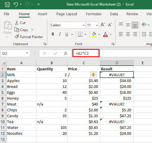
For example, you’re using a formula that calculates numbers. If there is a text string in one of the referenced cells, the formula won’t work. Instead of the result, you’ll see the #VALUE error in the selected blank cell.

The perfect example is when you’re trying to perform a simple mathematical calculation such as addition or multiplication, and one of the values is not numeric.

There are several ways to fix this error:

• Manually enter the missing numbers.
• Use an Excel function that ignores the text strings.
• Write an IF statement.

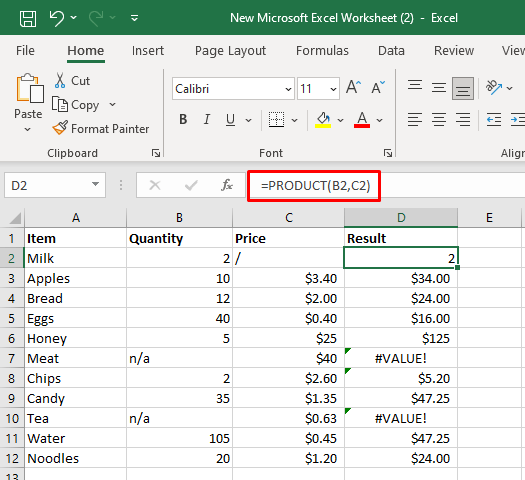
In the example above we can use the PRODUCT function: =PRODUCT(B2,C2).

This function will ignore the cells with empty spaces, incorrect data types, or logical values. It’ll give you a result as if the referenced value was multiplied by 1.

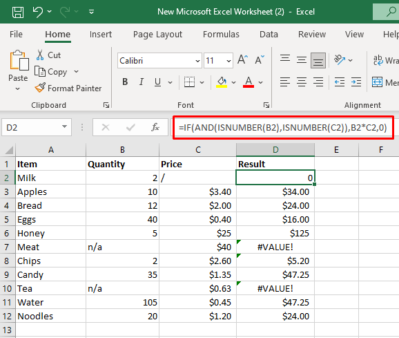
You can also build an IF statement that’ll multiply two cells if they are both containing numeric values. If not, the return will be zero. Use the following:

=IF(AND(ISNUMBER(B2),ISNUMBER(C2)),B2*C2,0)

Fix #VALUE Error Caused by Spaces and Hidden Characters

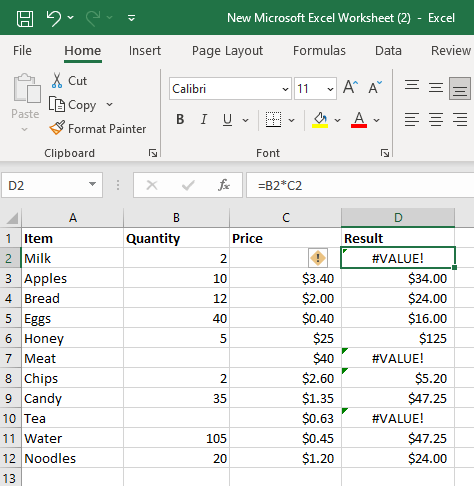
Some formulas can’t work if some of the cells are filled with hidden or invisible characters or spaces. Even though visually these cells look empty, they may contain a space or even a non-printing character. Excel considers spaces as text characters, and as in the case of different data types, this might cause the #VALUE Excel error.

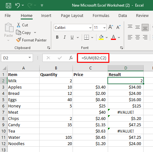
In the example above, the C2, B7, and B10 cells seem empty, but they contain several spaces which are causing the #VALUE error when we try to multiply them.

To tackle the #VALUE error you’ll have to make sure the cells are empty. Select the cell and press the DELETE key on your keyboard to remove any invisible characters or spaces.

You can also use an Excel function that ignores text values. One such is the SUM function:

=SUM(B2:C2)

Fix #VALUE Error Caused by Incompatible Ranges

If you’re using functions that accept multiple ranges in their arguments, won’t work if those ranges are not of the same size and shape. If that’s the case, your formula will result in the #VALUE error. Once you change the range of cell references the error should disappear.

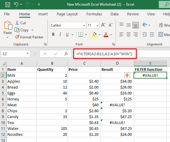
For example, you’re using the FILTER function and you’re trying to filter the range of cells A2:B12 and A3:A10. If you use the =FILTER(A2:B12,A2:A10=”Milk”) formula, you’ll get the #VALUE error.

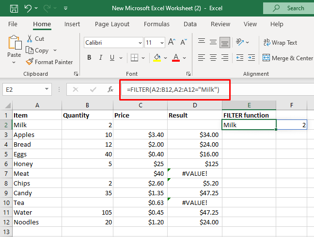
You’ll need to change the range to A3:B12 and A3:A12. Now that the range is of the same size and shape, your FILTER function won’t have a problem calculating.

Fix #VALUE Error Caused by Incorrect Date Formats

Microsoft Excel can recognize different date formats. But you might be using a format that Excel cannot recognize as a date value. In such a case, it’ll treat it as a text string. If you try using these dates in formulas, they’ll return the #VALUE error.

The only way to deal with this issue is to convert the incorrect date formats to the correct ones.

Fix #VALUE Error Caused by Incorrect Formula Syntax

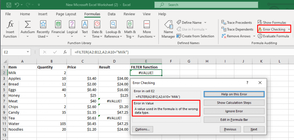
If you’re using the wrong formula syntax while trying to make your calculations, the result would be the #VALUE error. Luckily, Microsoft Excel has Auditing Tools that’ll help you with the formulas. You’ll find them in the Formula Auditing group in the ribbon. Here’s how to use them:

1. Select the cell with the formula that returns the #VALUE error.
2. Open the Formulas tab in the ribbon.

3. Under the Formula Auditing group find and select Error Checking, or Evaluate Formula.

Excel will analyze the formula you used in that particular cell, and if it finds a syntax error it’ll get highlighted. The detected syntax error can be easily corrected.

For example, if you’re using =FILTER(A2:B12,A2:A10=”Milk”) you’ll receive the #VALUE error because the range values are incorrect. To find where the problem is in the formula, click the Error Checking and read the results from the dialog box.

Correct the formula syntax to read =FILTER(A2:B12,A2:A12=”Milk”) and you’ll fix the #VALUE error.

Fix #VALUE Error in Excel XLOOKUP and VLOOKUP Functions

If you need to search and retrieve data from your Excel worksheet or the workbook, you’ll commonly use the XLOOKUP function, or its modern successor the VLOOKUP function. These functions can also return the #VALUE error in some cases.

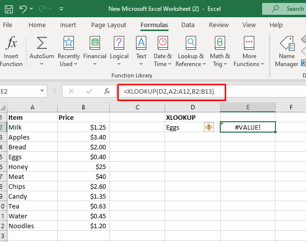
The most common cause of the #VALUE error in XLOOKUP is the incomparable dimensions of the return arrays. It can also happen when the LOOKUP array is bigger or smaller than the return array.

For example, if you’re using the formula: =XLOOKUP(D2,A2:A12,B2:B13), the return will be the #VALUE error because lookup and return arrays contain a different number of rows.

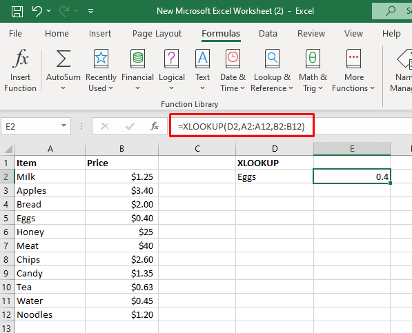
Adjust the formula to read: =XLOOKUP(D2,A2:A12,B2:B12).

Use IFERROR or IF Function to Resolve the #VALUE Error

There are formulas you can use in order to handle the errors. When it comes to #VALUE errors, you can use the IFERROR function or the combination of IF and ISERROR functions.

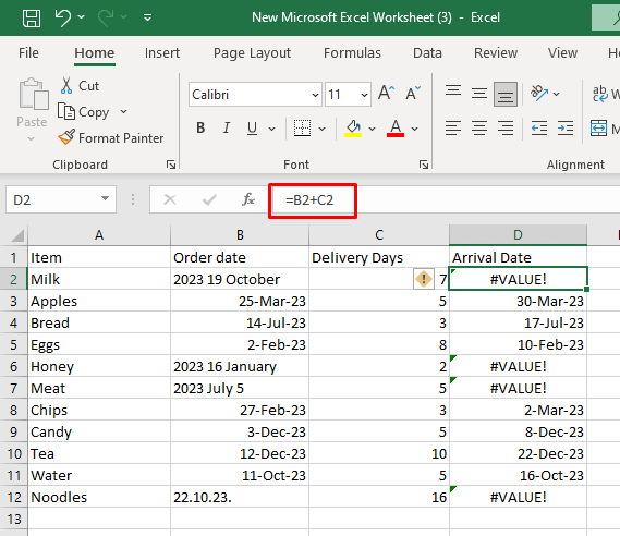
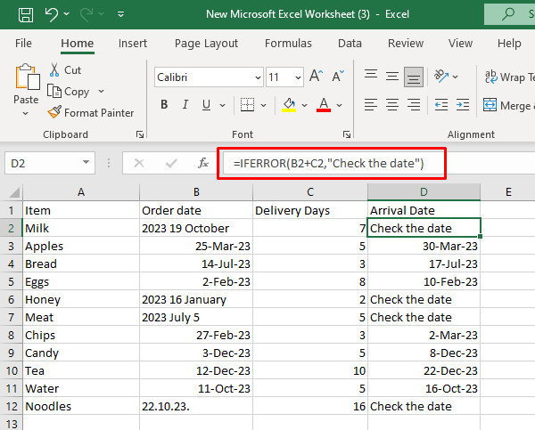
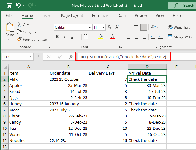
For example, you can use the IFERROR function to replace the #VALUE error with a more meaningful text message. Let’s say you want to calculate the arrival date in the example below, and you want to replace the #VALUE error caused by the incorrect date format, with the “Check the date” message.

You’ll use the following formula: =IFERROR(B2+C2,”Check the date”).

In case there is no error, the above formula will return the result of the first argument.

The same can be achieved if you use the combination of the IF and ISERROR formula:

=IF(ISERROR(B2+C2),”Check the date”,B2+C2).

This formula will first check if the return result is an error or not. If it is an error it’ll result in the first argument (Check the date), and if not, it’ll result in the second argument (B2+C2).

The only drawback of the IFERROR function is that it’ll catch all types of errors, not just the #VALUE one. It won’t make a difference between errors such as the #N/A error, #DIV/0, #VALUE, or #REF.

Excel, with its wealth of functions and features, offers endless possibilities for managing and analyzing data. Understanding and conquering the #VALUE! error in Microsoft Excel is a vital skill in the world of spreadsheet wizardry. These little hiccups can be frustrating, but armed with the knowledge and techniques from this article, you’re well-prepared to troubleshoot and resolve them.