Drop-down lists in Excel are powerful tools. They let you provide users with a drop-down arrow that, when selected, provides them with a list of choices.
This can reduce data-entry errors because it avoids users from having to type answers directly. Excel even lets you pull the items for those drop-down lists from a range of cells.
However, it doesn’t stop there. Using some creative ways to configure data validation for drop-down cells, you can even create multiple, linked drop-down lists, where the items that are available in a second list depend on the section the user made in the first list.
What Are Multiple Linked Drop-Down Lists Good For?
Consider that most forms online fill out secondary drop-down lists based on what you answer in the drop-down list before it. This means you can make your Excel data-entry sheets just as advanced as online forms. It will modify itself based on the user’s answers.
For example, let’s say you’re using an Excel spreadsheet to collect computer information from your users who need computer repairs.
The entry options might look like this:
- Computer Part: Monitor, Mouse, Keyboard, Base System
- Part Type:
- Monitor: Glass, Housing, Power Cord, Internal Electronics
- Mouse: Wheel, LED Light, Cord, Buttons, Casing
- Keyboard: Keys, Housing, Membrane, Cord, Internal Electronics
- Base System: Casing, Buttons, Ports, Power, Internal Electronics, Operating System
As you can see from this tree, the information that should be available to select for “Part Type” depends on which Computer Part the user selects in the first dropdown list.
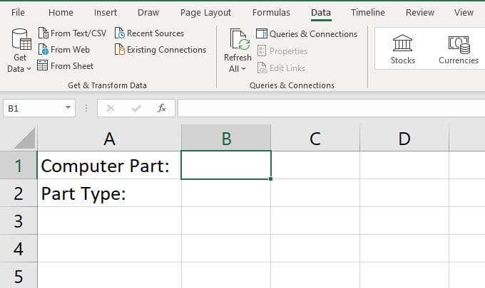
In this example, your spreadsheet may start out looking something like this:
If you create multiple, linked drop-down lists, you can use the item selected from the drop-down list in B1 to drive the contents of the drop-down list in B2.
Let’s take a look at how you can set this up. Also, feel free to download our example Excel sheet with the example below.
Create Your Drop-Down List Source Sheet
The cleanest way to set something like this up is to create a new tab in Excel where you can configure all of your drop-down list items.
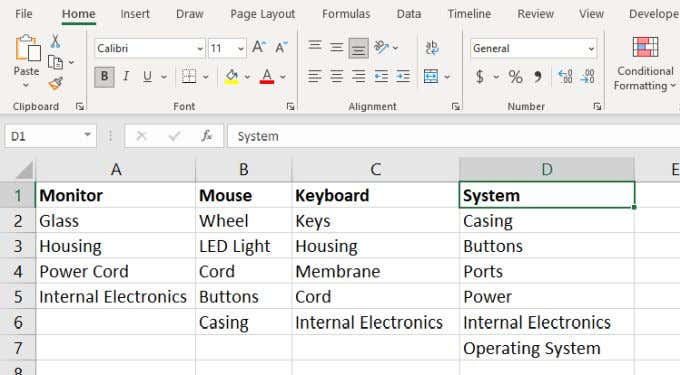
To set up these linked drop-down lists, create a table where the header at the top are all of the computer parts you want to include in the first dropdown list. Then list all of the items (part types) that should go under that header.
Next, you’ll want to select and name each range so that when you’re setting up Data Validation later, you’ll be able to select the correct one.
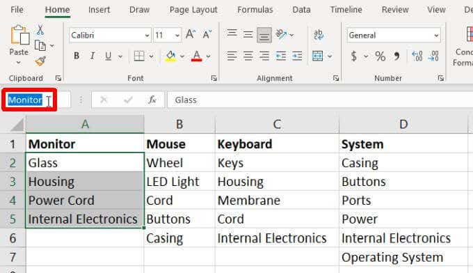
To do this, select all of the items under each column and name that selected range the same as the header. To name a table, you simply type the name in the field over the “A” column.
For example, select cells A2 through A5, and name that range “Monitor”.
Repeat this process until you have all of the ranges named appropriately.
An alternative way to do this is using Excel’s Create from Selection feature. This lets you name all of the ranges like the manual process above, but with a single click.
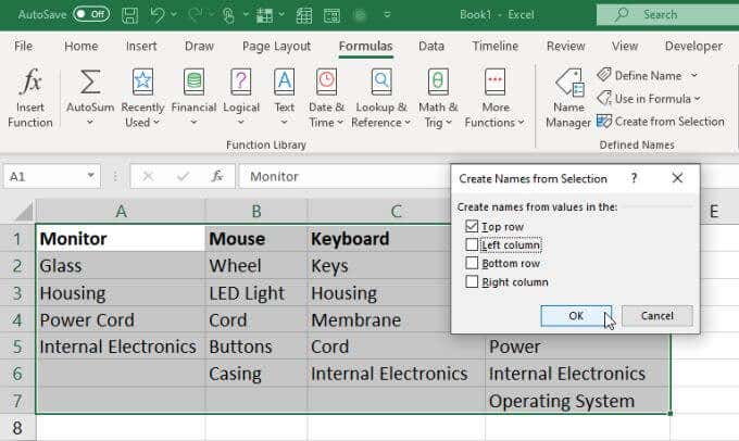
To do this, just select all of the ranges in the second sheet that you created. Then select Formulas from the menu, and select Create from Selection in the ribbon.
A pop-up window will appear. Make sure only Top row is selected and then select OK.
This will use the header values in the top row to name each of the ranges underneath it.
Set Up Your First Drop Down List
Now it’s time to set up your multiple, linked drop-down lists. To do this:
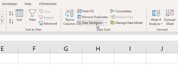
1. Back on the first sheet, select the blank cell to the right of the first label. Then select Data from the menu, and select Data Validation in the ribbon.
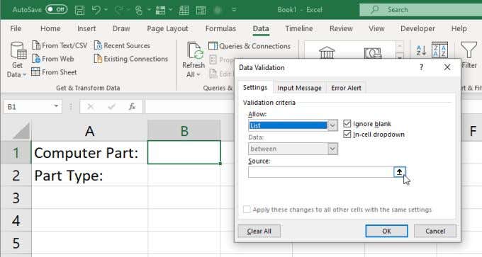
2. In the Data Validation window that opens, select List under Allow, and under Source, select the up arrow icon. This will let you select the range of cells you want to use as the source for this drop-down list.
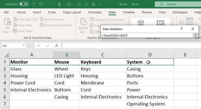
3. Select the second sheet where you set up the drop-down list source data, and then select only the header fields. These will be used to fill out the initial drop-down list in the cell you’ve selected.
4. Select the down arrow in the selection window to expand the Data Validation window. You’ll see the range you’ve selected now displayed in the Source field. Select OK to finish.
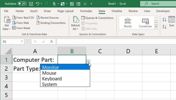
5. Now, back on the main sheet, you’ll notice that the first drop-down list contains each of the header fields from the second sheet.
Now that your first drop-down list is finished, it’s time to create your next, linked drop-down list.
Set Up Your First Drop Down List
Select the second cell that you want to load list items for depending on what’s selected in the first cell.
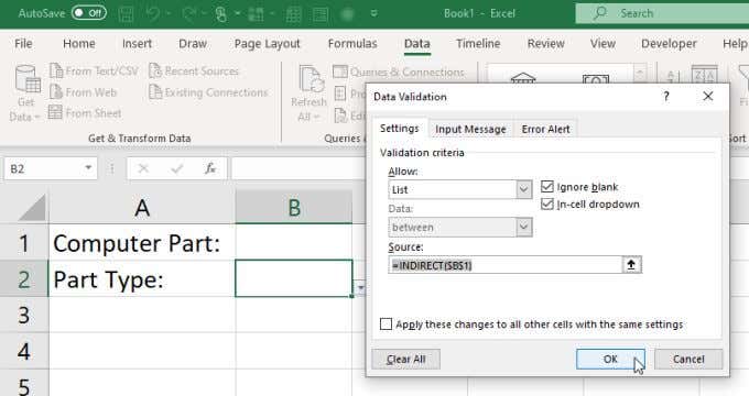
Repeat the process above to open the Data Validation window. Select List in the Allow drop-down. The Source field is what will pull in list items depending on what’s selected in the first drop-down list.
To do this, enter the following formula:
=INDIRECT($B$1)
How does the INDIRECT function work?
This function returns a valid Excel reference (in this case to a range), from a text string. In this case, the text string is the name of the range passed by the first cell ($B$1). So INDIRECT takes the name of the range and then provides the drop-down data validation with the correct range associated with that name.
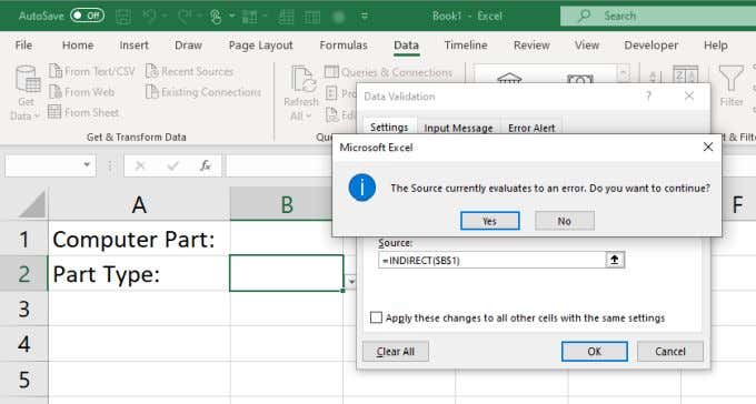
Note: If you configure the data validation for this second drop-down without selecting a value from the first drop-down, you’ll see an error message. You can select Yes to ignore the error and continue.
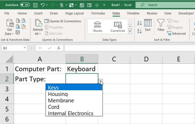
Now, test your new multiple, linked drop-down lists. Use the first drop-down to select one of the computer parts. When you select the second drop-down, you should see the appropriate list items for that computer part. These were the part types in the column on the second sheet that you filled in for that part.
Using Multiple Linked Drop-Down Lists in Excel
As you can see, this is a very cool way to make your spreadsheets much more dynamic. By filling in subsequent drop-down lists in response to what users select in other cells, you can make your spreadsheets far more responsive to users, and the data far more useful.
Play around with the tips above and see what kind of interesting linked drop-down lists you can create in your spreadsheets. Share some of your own interesting tips in the comments section below.

