Microsoft Excel is an excellent tool for storing and analyzing data. It offers a wide range of statistical tools and formulas, making it easy to determine key statistics for different datasets. In this article, we’ll explain how to calculate standard error in Excel (and what it is in the first place).
What Is Standard Error?
Standard error lets you see how accurately sample data fits a larger dataset. In other words, it calculates how accurate a distribution of data is to the entire population.
It does this by calculating standard deviation, which is how far the average of your sample deviates from the average of the entire dataset.
The formula for standard error is:
Where is the standard deviation for the entire dataset and is the square root of the sample size.
To illustrate the concept of standard error with an example, imagine a school with 500 students. We want to estimate the average height of the students, so we select 30 students and measure them. The average height of this sample is 160 cm.
However, if we take a sample of another 30 students, we find that the average height is 152 cm.
The variation of these sample averages against the actual population average is the standard error. The smaller the standard error, the more representative the sample mean is of the population. The larger the error, the less representative it is and the more variable the data is.
How to Calculate Standard Error in Excel
Microsoft Excel provides built-in formulas for calculating standard deviation and the square root of a set of numbers, making it very easy to calculate standard error. Here’s how to use these formulas, using a simple example:
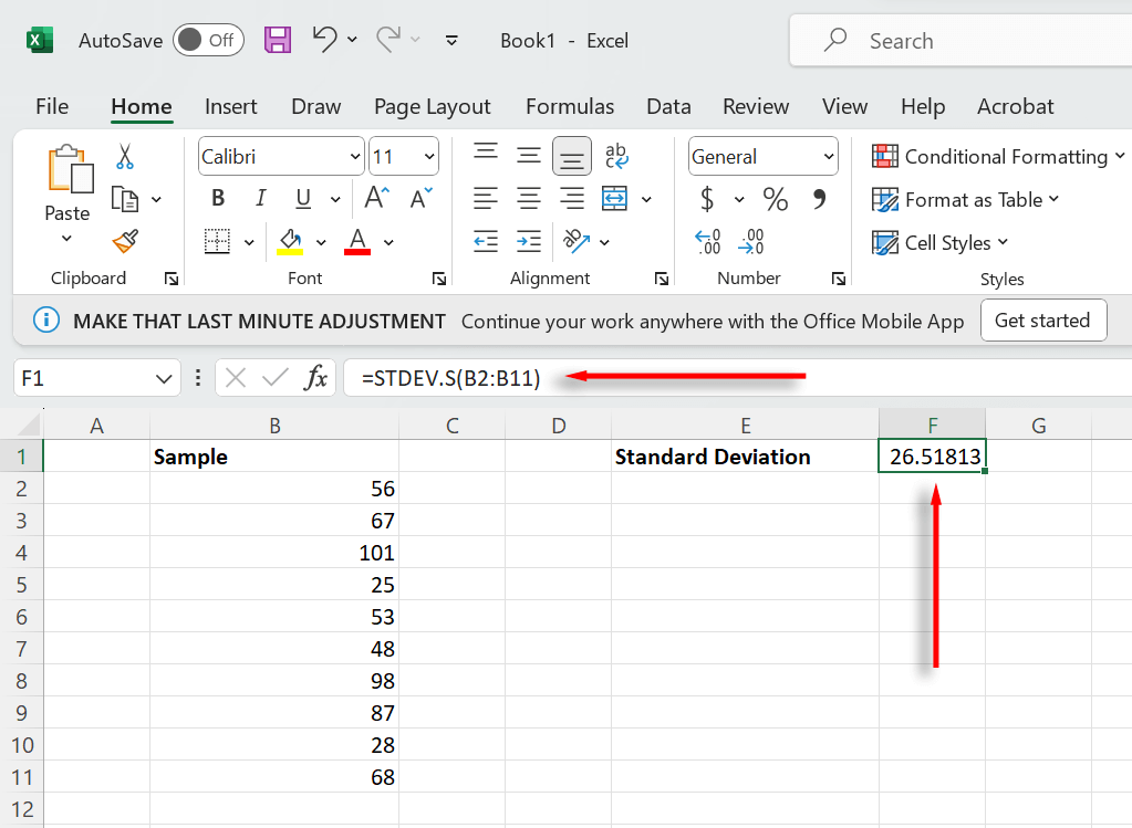
- Organize your data into a column as below.
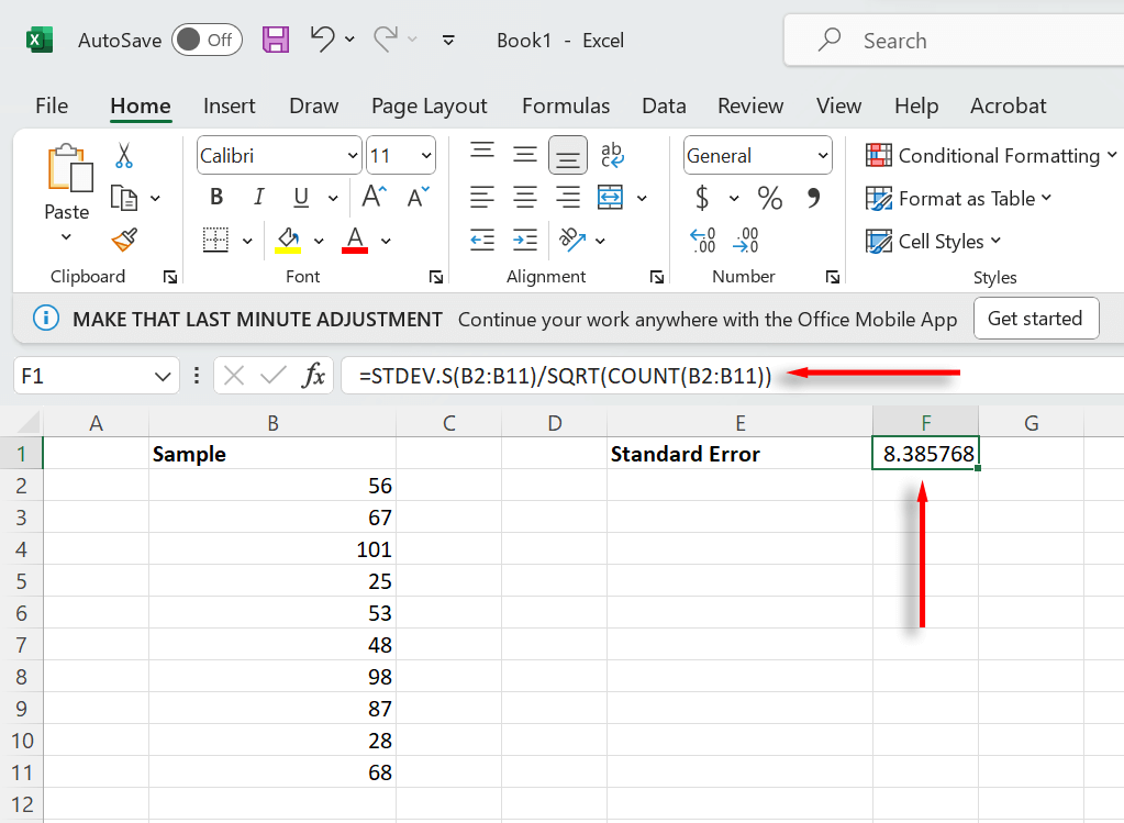
- First, we need to calculate the standard deviation of your sample. To do so, select a cell, then type =STDEV.S(B2:B11) (selecting your sample range) and press Enter. Make sure to use STDEV.S as this returns the standard deviation for a sample, rather than an entire population.
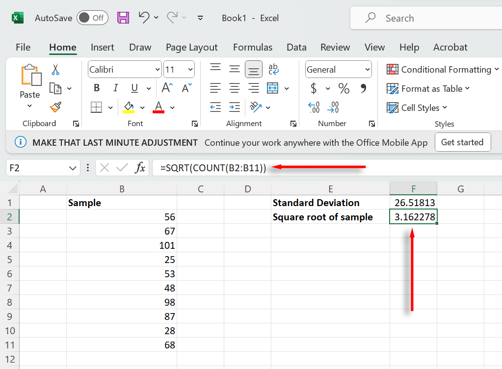
- Next, we need to calculate the square root of the sample size. To do so, select a second cell and type SQRT(COUNT(B2:B11)) (selecting your sample range). Then, press Enter.
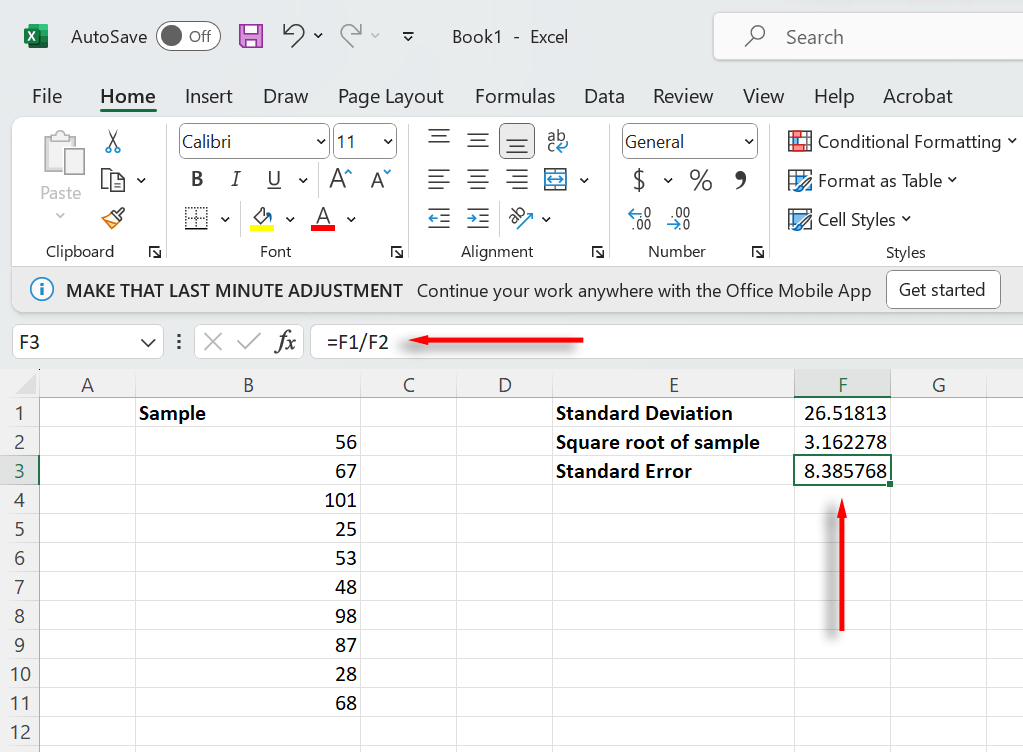
- Finally, we need to divide the standard deviation by the square root of the sample size. Select a third cell and type =F1/F2, selecting the cells that represent each value. Press Enter.
The cell should now display the standard error of your sample. You can combine both of these formulas into one equation. Simply type =STDEV(B2:B11)/SQRT(COUNT(B2:B11)) (selecting your data range instead of A1:A10).
Note: Make sure to follow the correct function syntax to ensure that your formulas work as designed. If you aren’t sure about the syntax, you can separate each part of the standard error formula and divide them into a third cell.
Err On the Side of Caution
Microsoft Excel is a powerful tool for statistical analysis. It can also be used to calculate other forms of variance and loan repayments – and that’s not all. Hopefully, you’re now able to calculate standard error and you can get on to the next part of your analysis.
