
Your PivotTable shows “Sum of Sales” in dollars, but you need to show those values as percentages, such as each region’s share of the company or each salesperson’s share of their region. Excel’s Show Values As feature does this in a few clicks, with no formulas.
What Is Show Values As?
Show Values As is a setting on any PivotTable value field. It keeps the underlying sum and changes what the cell displays. Each option divides by a different number. % of Grand Total divides by everything. % of Row Total divides by the row. % of Parent Row Total divides by the group directly above. That’s why the same data can give three different answers. It’s available in Excel for Windows, Excel for Mac, and Excel for the web, but the menus differ slightly on Mac and the web (Step 2 covers each).
Prerequisites
- Excel for Windows or Mac (Microsoft 365, Excel 2021, or Excel 2024), or Excel for the web (free with a Microsoft account)
- A dataset with at least one number column and one or more category columns
- A basic idea of how to drag fields into Rows and Values. If you’re new to this, start with Microsoft’s guide on how to create your first PivotTable in Excel.
This article uses the small dataset below throughout. Type it into cells A1:D9 to follow along.
| Region | Salesperson | Quarter | Sales |
|---|---|---|---|
| East | Ana | Q1 | 6000 |
| East | Ana | Q2 | 4000 |
| East | Ben | Q1 | 4000 |
| East | Ben | Q2 | 6000 |
| West | Cara | Q1 | 10000 |
| West | Cara | Q2 | 10000 |
| West | Dev | Q1 | 5000 |
| West | Dev | Q2 | 5000 |
East sells $20,000 and West sells $30,000, for a grand total of $50,000.
Step-by-Step Guide
Step 1: Build the Example PivotTable
- Click any cell inside your data.
- Go to Insert > PivotTable, confirm the range, choose New Worksheet, and click OK.
- In the PivotTable Fields pane, drag Region to Rows.
- Drag Salesperson to Rows, below Region.
- Drag Sales to Values.
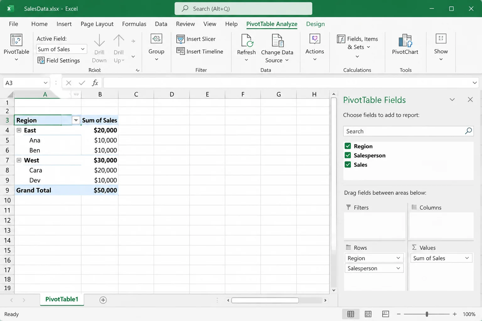
Expected result: East shows $20,000 (Ana $10,000, Ben $10,000). West shows $30,000 (Cara $20,000, Dev $10,000). The Grand Total is $50,000.
Step 2: Open the Show Values As Menu
You can reach Show Values As in two ways. The right-click menu is fastest. Value Field Settings gives you every option, plus renaming and number formatting.
On Windows
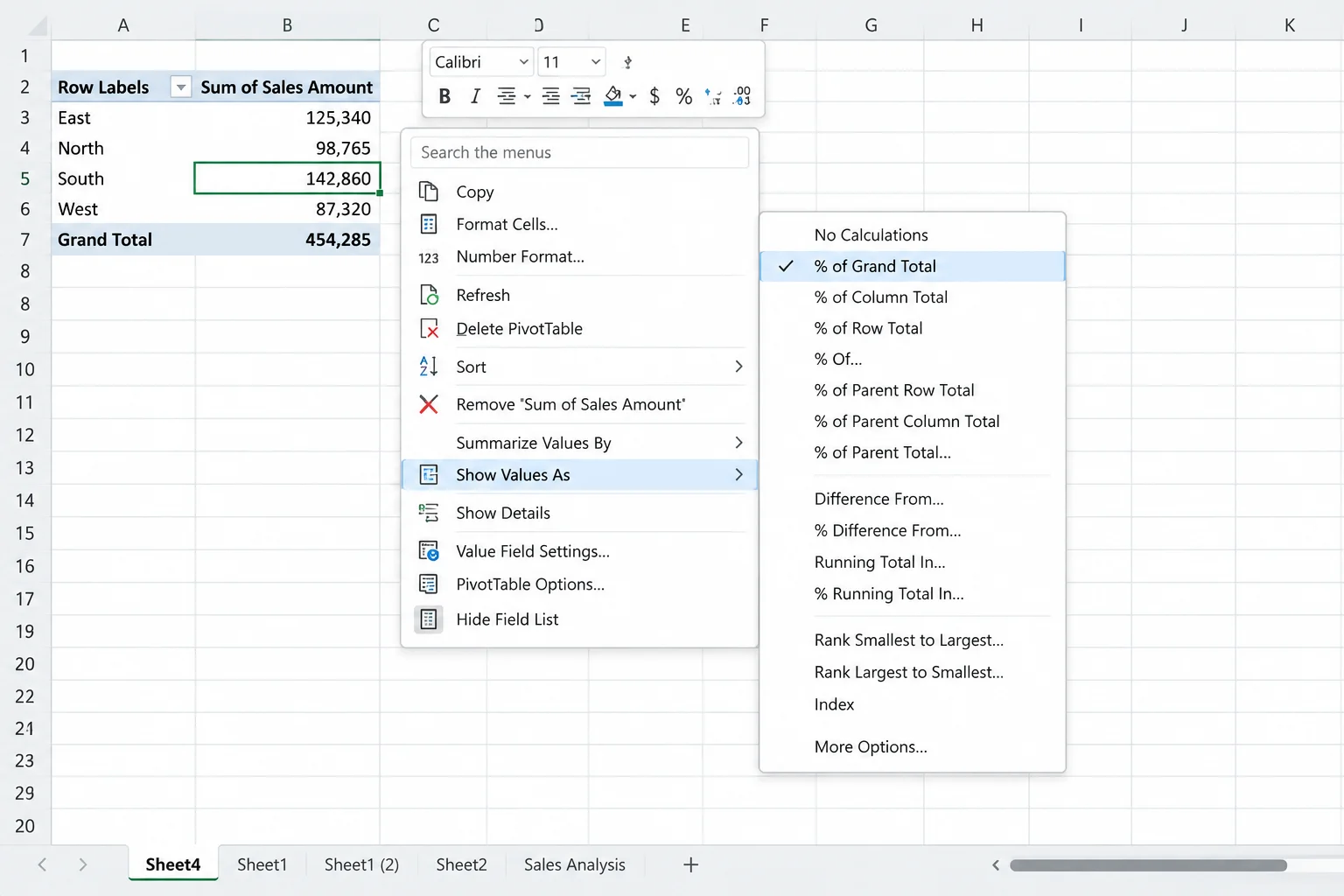
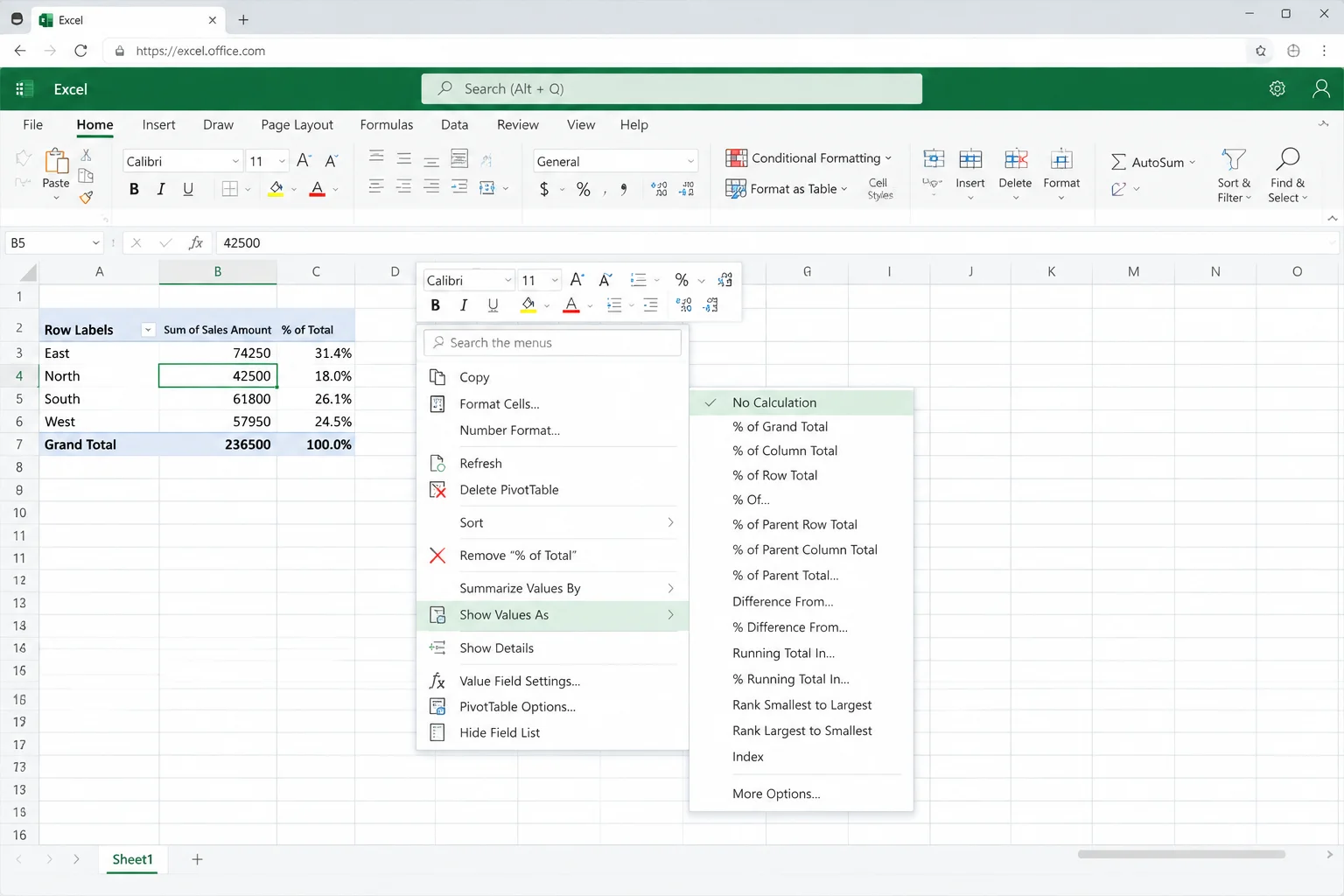
- Right-click any number in the Sum of Sales column. Don’t right-click a label like “East.”
- Hover over Show Values As to open the submenu.
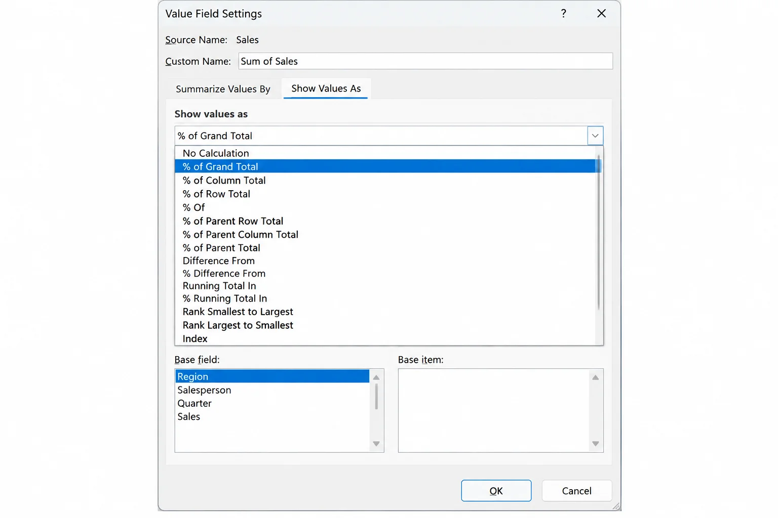
- For the full dialog instead, click a value cell and go to PivotTable Analyze > Field Settings. You can also right-click a value and choose Value Field Settings.
- Click the Show Values As tab and open the Show values as dropdown.
On macOS
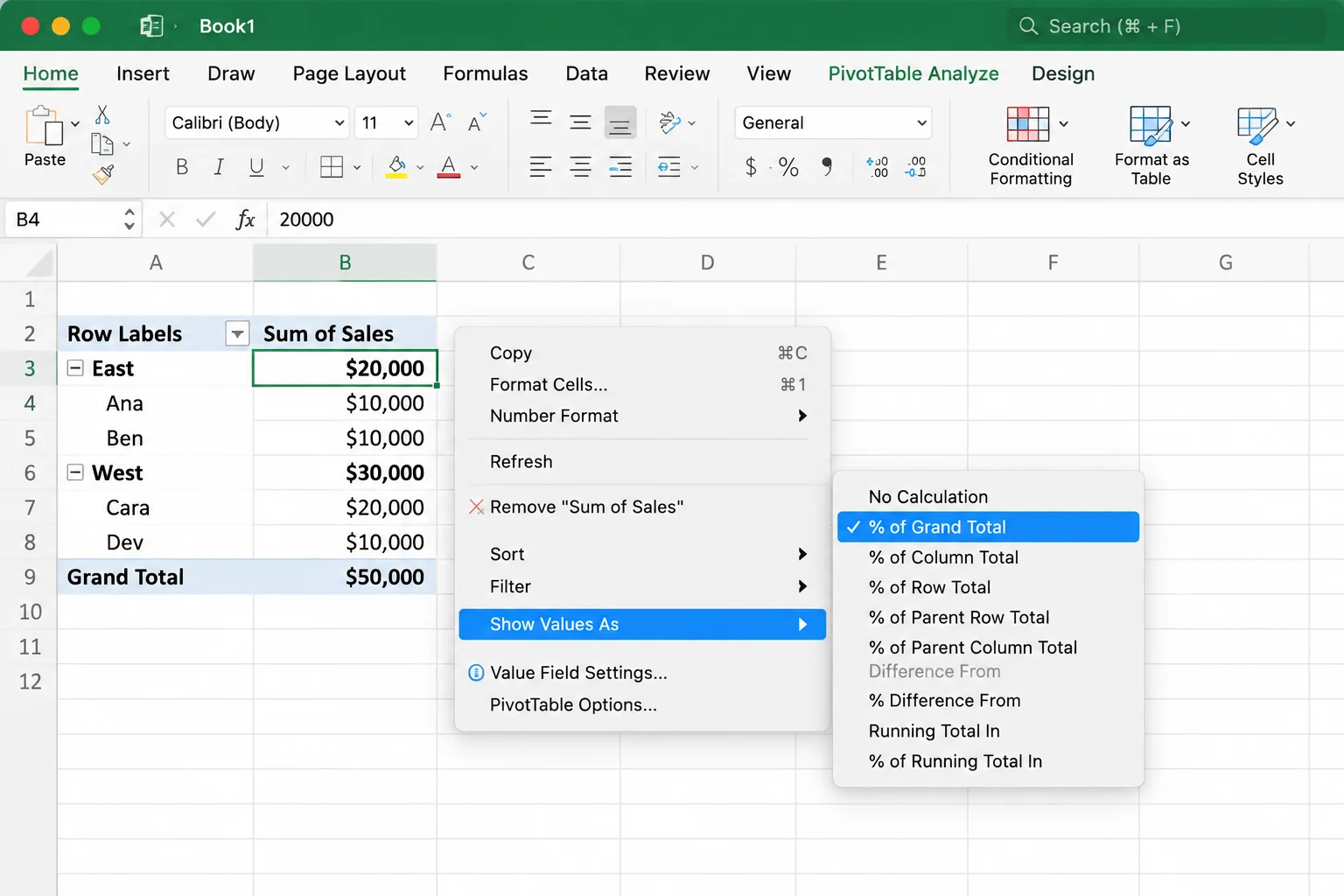
- Control-click or right-click a number in the Sum of Sales column.
- Hover over Show Values As and choose an option. The Mac menu doesn’t list every option that Windows shows. If the one you want is missing, choose More Options.
- For the dialog, right-click a value and choose Field Settings. On a Mac, the percentage choices sit on the Show data as tab.
On Excel for the web
- Open the workbook at office.com and click a value in the PivotTable.
- Right-click the value and hover over Show Values As.
- Pick an option from the list. For % of Parent Total, hover over it and choose the parent field to divide by. The web version has fewer dialogs than desktop Excel, so if an option in this guide isn’t offered, use the desktop app.
Step 3: Show Each Item’s Share With % of Grand Total
This option answers the question “What share of all company sales is this?”
- Right-click a Sum of Sales value.
- Choose Show Values As > % of Grand Total.
Expected result:
| Row | % of Grand Total |
|---|---|
| East | 40.00% |
| Ana | 20.00% |
| Ben | 20.00% |
| West | 60.00% |
| Cara | 40.00% |
| Dev | 20.00% |
| Grand Total | 100.00% |
Step 4: Use % of Column Total and % of Row Total
These two options only matter when you have fields in both Rows and Columns.
- Drag Quarter from the field list into Columns.
- Right-click a value and choose Show Values As > % of Column Total.
Each quarter’s column now adds up to 100%. In Q1, Ana shows 24% ($6,000 of Q1’s $25,000), Cara shows 40%, and West shows 60%. This answers “Who drove Q1?”
- Right-click a value again and choose Show Values As > % of Row Total.
Each row now adds up to 100% across the quarters. Ana shows 60% in Q1 and 40% in Q2. Cara shows 50% and 50%. This answers “When did each person make their sales?”
The difference in one line: % of Grand Total divides by $50,000. % of Column Total divides by that column’s total. % of Row Total divides by that row’s total.
Step 5: Show Each Salesperson’s Share of Their Region With % of Parent Row Total
This option answers “How much of my region did each rep bring in?”
- Drag Quarter out of Columns so only Region and Salesperson remain in Rows.
- Right-click a value and choose Show Values As > % of Parent Row Total.
Expected result: Each salesperson is divided by their own region’s subtotal, so Ana shows 50%, Ben 50%, Cara 66.67%, and Dev 33.33%. Each region row is divided by the grand total, so East shows 40% and West shows 60%. The Grand Total row shows 100%.
Compare Cara’s numbers. She is 40% of the company but 66.67% of West. Both numbers are correct. They answer different questions.
Two related options:
- % of Parent Column Total does the same thing for nested fields in the Columns area.
- % of Parent Total… asks for a Base field. Pick Region to divide every salesperson by their region subtotal. Use this when you have three or more levels and want to skip a level.
Step 6: Compare Against a Benchmark With % Of
- Remove Salesperson from Rows so only Region is left.
- Right-click a value and choose Show Values As > % Of…
- Set Base field to Region and Base item to East. Click OK.
Expected result: East shows 100% and West shows 150%. West sold one and a half times what East sold.
Step 7: Track Cumulative Progress With % Running Total In
- Drag Quarter back into Columns.
- Right-click a value and choose Show Values As > % Running Total In…
- Set Base field to Quarter and click OK.
Expected result: East, West, and the Grand Total each show 50% in Q1 and 100% in Q2. (If you add Salesperson back under Region, Ana shows 60% in Q1 and Ben shows 40%, because their quarters weren’t even.) This is useful for “how far through the year’s total are we?” If you work with real dates, group them into months or quarters first.
Step 8: Show the Dollar Amount and the Percentage Side by Side
Show Values As replaces the dollar figures. To keep both, add the field twice.
- Reset the layout. Put Region and Salesperson in Rows and leave Columns empty.
- Drag Sales into Values a second time. You’ll see Sum of Sales and Sum of Sales2.
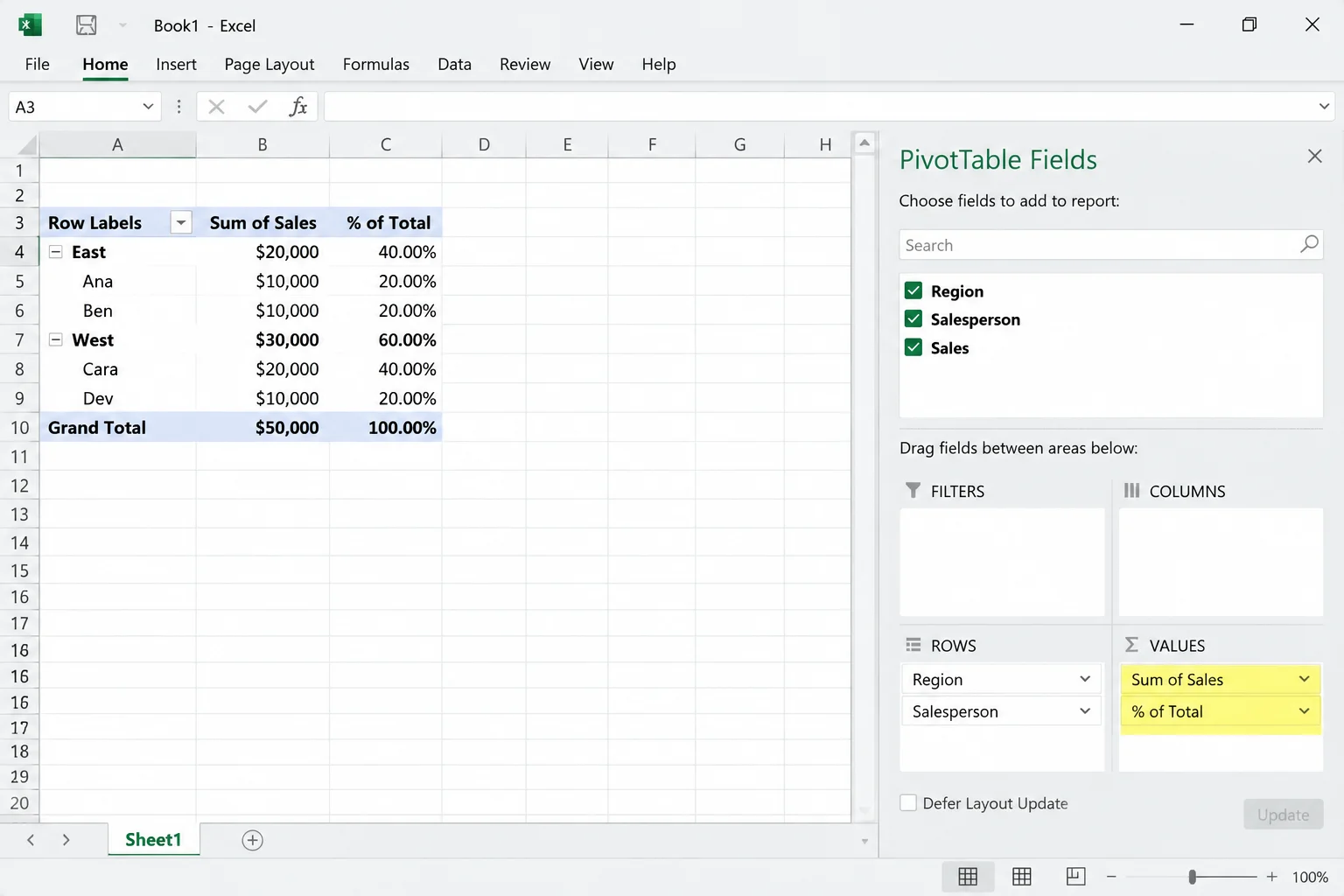
- Right-click a number in the Sum of Sales2 column and choose Value Field Settings.
- In Custom Name, type
% of Total. - On the Show Values As tab, choose % of Grand Total and click OK.
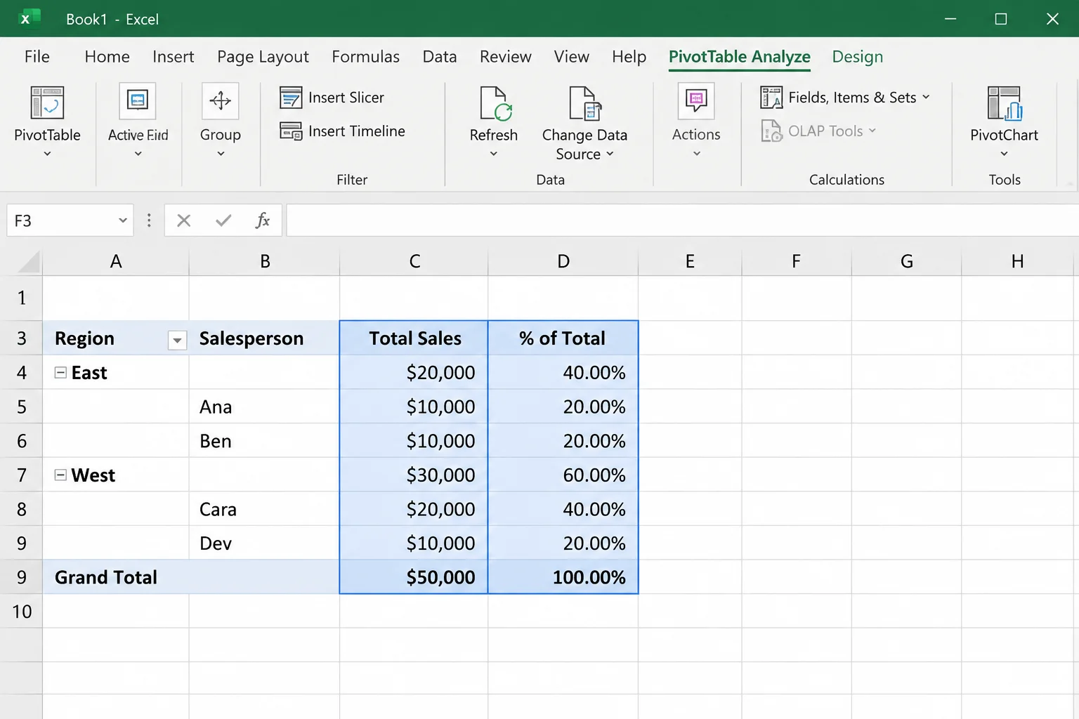
- Rename the first field to
Total Salesthe same way.
Step 9: Format the Percentages
Excel usually applies percentage formatting on its own. If you see 0.4 instead of 40%, or you want fewer decimals, fix it at the field level.
- Right-click the percentage column and choose Value Field Settings.
- Click Number Format.
- Choose Percentage and set Decimal places to
1or0.
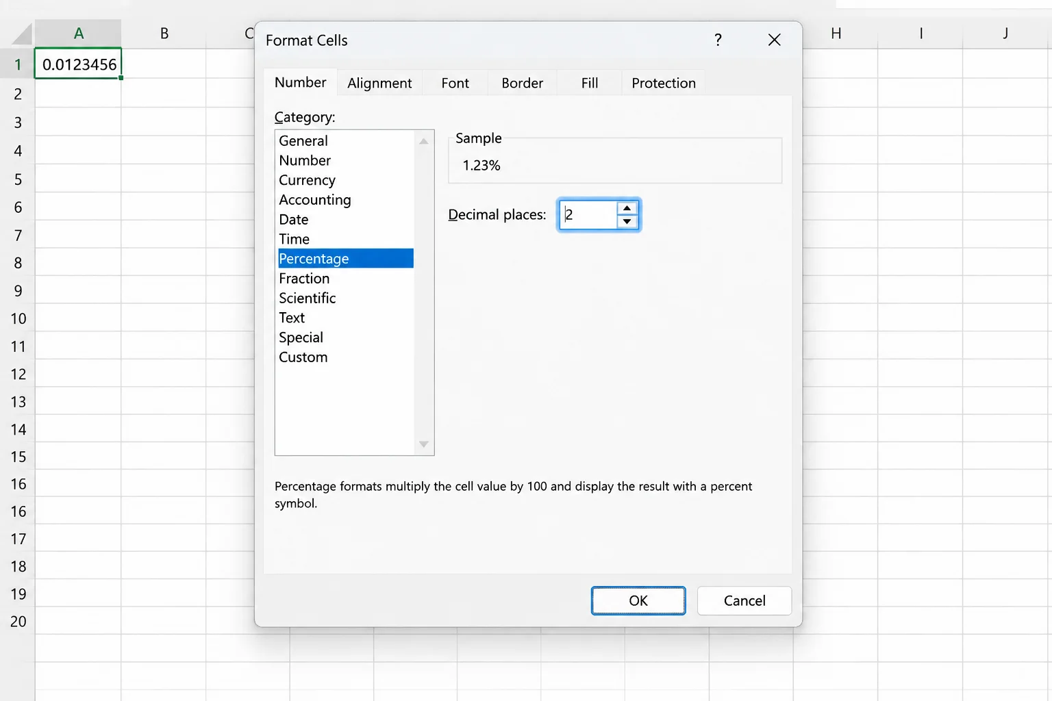
- Click OK twice.
Setting the format in Value Field Settings changes the number format for the entire field. In Excel for the web, if the Number Format button isn’t there, select the column and use Home > Number Format > Percentage.
Configuration
| Setting | Where | Default | When to change it |
|---|---|---|---|
| Show values as | Value Field Settings > Show Values As | No Calculation | Any time you want percentages |
| Base field / Base item | Same tab, below the dropdown | Unused | Required for % Of, % of Parent Total, and % Running Total In |
| Custom Name | Top of Value Field Settings | Sum of Sales | When the same field appears twice |
| Number Format | Button in Value Field Settings | Depends on the option | For decimals or percent display |
To match your business question to the right option:
- For “share of everything,” use % of Grand Total.
- For “share within a group,” use % of Parent Row Total.
- For “share within a row or column of a grid,” use % of Row Total or % of Column Total.
Tips and Troubleshooting
Fix #1: Refresh the PivotTable
Percentages look stale when the source data changed but the PivotTable didn’t update. Microsoft is adding an Auto Refresh option for PivotTables built on data in the same workbook (currently for Microsoft 365 Insiders). Without it, a PivotTable keeps showing old numbers until you refresh it.
- Right-click anywhere in the PivotTable.
- Choose Refresh, or press
Alt + F5on Windows. - To update every PivotTable in the workbook at once, go to PivotTable Analyze, select the arrow under Refresh, and choose Refresh All.
If refreshing doesn’t help, see our guide on how to fix a PivotTable that’s not calculating or updating.
Fix #2: Right-Click a Value, Not a Label
Microsoft’s steps for Show Values As all start from a value cell. If you don’t see it in the menu, you most likely right-clicked a row label, a column header, or a blank cell.
- Click a number inside the Values area.
- Right-click that same cell.
Fix #3: Clear Filters When Percentages Don’t Add Up to 100%
Percentages are calculated from the data the PivotTable currently includes. Report filters, unchecked items in the label filters, and hidden items all change the total, so a column can show 100% even though part of your source data is left out.
- Check the Filters area and the filter arrows on Row Labels and Column Labels for anything unchecked.
- Go to PivotTable Analyze > Clear > Clear Filters if you want the full dataset.
- Confirm Design > Grand Totals and Subtotals are turned on so you can check the 100% row.
Small differences like 99.99% are rounding. Add a decimal place in Step 9 to confirm.
Fix #4: Pick a Base Item That Exists Everywhere to Stop #N/A
You’ll see “#N/A” with % Of when the base item doesn’t exist for a row. In our example, leave Salesperson in Rows and set the base to East. Cara’s row then shows “#N/A” because Excel looks for Cara in East and finds no such person.
- Remove the nested field (Salesperson), or
- Choose a base item that appears under every row, or
- Switch to % of Grand Total or % of Parent Row Total, which don’t need a base item.
Fix #5: Stack Fields for Parent Percentages
% of Parent Row Total looks identical to % of Grand Total when Rows holds only one field.
- Make sure at least two fields are in Rows.
- Drag them into the order you want, such as Region above Salesperson.
Fix #6: Change “Count of Sales” Back to “Sum of Sales”
If Excel reads any of your Sales values as text, it summarizes the field as a count instead of a sum. That happens when the column has text-formatted numbers or stray text in it. Percentages built on a count won’t match your dollar totals.
- Check the Sales column in your source data for text entries or numbers stored as text, and fix them.
- Right-click a value in the PivotTable and choose Value Field Settings.
- On the Summarize Values By tab, choose Sum and click OK.
- Refresh the PivotTable, then reapply your Show Values As option if needed.
Conclusion
Most people only need % of Grand Total and % of Parent Row Total. Add the field twice so the dollars stay visible, and you have a report that answers both “share of company” and “share of team.” If your percentages keep going wrong after a refresh, check the source data for blank or text-formatted numbers before you blame the PivotTable.