How To Use Flash Fill In Excel

Trying to fill out cells in Excel that incorporate text or data from multiple other cells in a sheet can be a very time consuming process. This is especially true if there are hundreds or thousands of rows in the spreadsheet.

Once you know how to use Flash Fill in Excel correctly, you can let Excel do all of the heavy lifting. You just provide a couple of manual cell entries to help Excel understand exactly what you’re trying to do. Then, Excel does the rest of the work for the rest of the spreadsheet.

If this sounds like a time-saving tip you’d like to try, let’s take a look at how you can use this feature to improve your own productivity.

Note: The Flash Fill feature in Excel is only available in Excel 2013 and later.

How To Use Flash Fill In Excel

The simplest application of Flash Fill in Excel is combining two words together. In the example below, we’ll show you how to use Flash Fill to quickly combine a first name and a last name into a third cell for the full name.

In this example, column C contains the first name, column D contains the last name, and column E is the column for the full name.

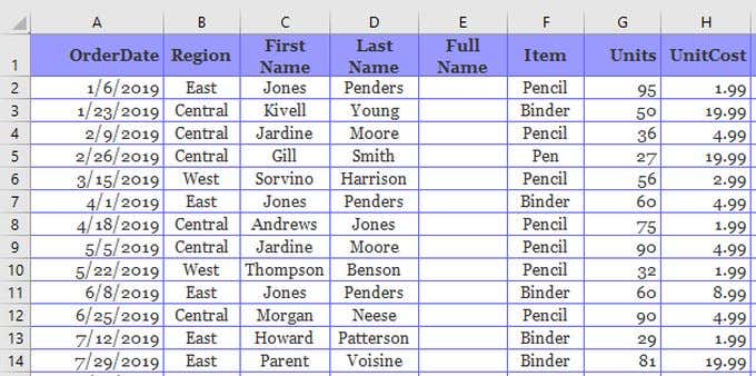
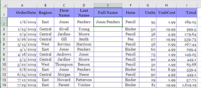
1. First, type the full name into the first cell the way you’d like it to look (combining the contents of the First Name cell and the Last Name cell.

2. After this, start typing the same thing into the next cell (the First Name and Last Name from the cells to the left). You’ll notice that Excel’s Flash Fill feature will automatically detect the pattern from the content of the cell above it that you typed manually.
   
   Using this “learning”, Excel will provide a preview of what it thinks you want to type. It will even show you how the rest of the cells will fill in for the rest of the column.

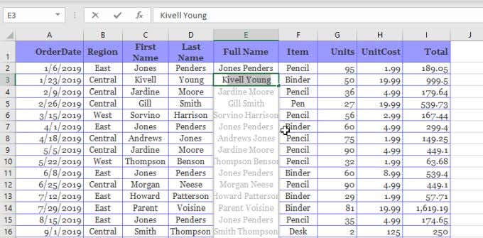
3. Just press Enter to accept this preview. You’ll see the Excel Flash Fill feature perform its magic as it fills in all of the rest of the cells in this column for you.

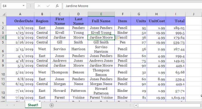
As you can see, the Flash Fill feature can save a tremendous amount of time if you compare manually typing one cell and Enter to having to manually type the names for all of the cells in the new column.

If you’ve noticed that the Flash Fill feature doesn’t work, you need to turn on the Flash Fill feature in Excel. You can see how to do that in the last section of this article.

Excel Flash Fill Options

When you perform the Flash Fill steps above, you’ll notice a small icon will appear next to the filled-in cells. If you select the drop-down arrow to the right of this icon, you’ll see some additional options you can use with the Flash Fill feature. 

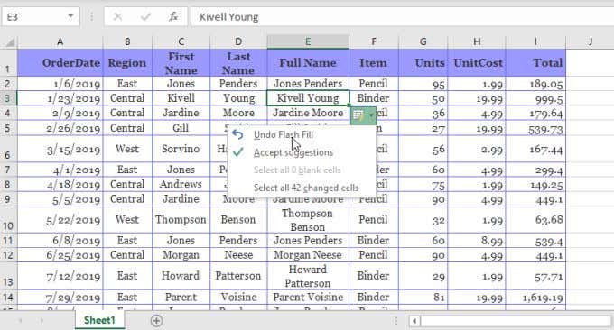
Using the Flash Fill options in this drop-down box, you can:

• Undo Flash Fill: Undo the action that filled in the entire column after you pressed Enter
• Accept suggestions: This will tell Excel’s Flash Fill feature for this column that you’re fine with the changes to the column and would like to keep them
• Select xx blank cells: Lets you identify any cells that didn’t get filled-in and are blank so that you can fix those if you need to
• Select xx changed cells: Lets you select all of the cells that automatically changed after the Flash Fill feature updated those cells

Once you select Accept suggestions, you’ll see that the “select” numbers for the “changed cells” will drop to zero. This is because once you accept the changes, those cell contents are no longer considered “changed” by the Flash Fill feature.

How To Enable Flash Fill In Excel

If you’ve noticed that Excel doesn’t provide a Flash Fill preview when you start typing the second cell, you may need to enable the feature.

To do this:

Select File > Options > Advanced. Scroll down to the Editing options section and make sure both Enable AutoComplete for cell values and Automatically Flash Fill are selected.

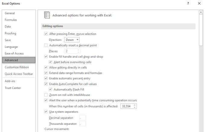
Select OK to finish. Now, the next time you start typing in the second cell after filling in the first, Excel should detect the pattern and provide you with a preview for how it thinks you want to fill in the rest of the cells in the column.

You can also activate the Flash Fill feature for the cell you have highlighted by selecting the Flash Fill icon in the Data menu under the Data Tools group in the ribbon. 

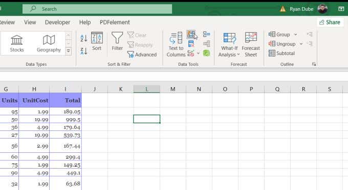
You can also use it by pressing Ctrl + E on the keyboard.

When To Use Flash Fill In Excel

Concatenating full names from two columns is a simple example of how you can use Flash Fill in Excel, but there are many more advanced uses for this powerful feature.

• Extract a substring from a large string (like a zip code from a full address) in another column
• Pull numbers out of alphanumeric strings
• Remove spaces from before or after strings
• Insert substrings (like a comma or dash) into existing strings
• Reformat dates
• Replace part of a string with new text

Keep in mind that, however useful the Flash Fill feature is, it will not automatically update when you change the original cells.

For example, in the first and last name example in the first section of this article, you could achieve the same output by using the Concatenate function and then filling the rest of the column with that function.

=CONCATENATE(C2,” “,D2)

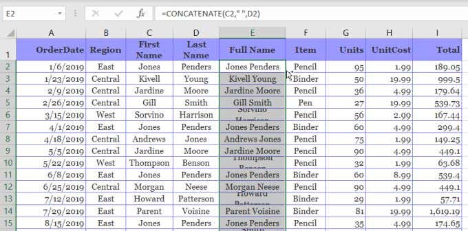
When you do this, if either of the first two cells change, the Full Name will update. One drawback of this is that if you delete either of the first two columns, the Full Name column will clear or display an error.

This is why the Flash Fill function in Excel is best used when you want to fully and permanently convert the original columns into a newly formatted string or number.