How to Use If and Nested If in Google Sheets

One of the most commonly used statements in nearly every programming language is the IF statement. So it should come as no surprise that using IF and nested IF statements in Google Sheets is very popular and very useful.

The IF statement in Google Sheets lets you insert different functions into a cell-based on conditions from other cells. When you nest IF statements, you can create more advanced analytics based on data. In this article, you’ll learn how to do this as well as see a few examples.

Using the IF Statement in Google Sheets

Before you can get fancy and start nesting IF statements, you need to understand how a simple IF statement works in Google Sheets first.

The easiest way to understand this is with an example. For our first example, imagine you pulled a list of mountains you’re thinking of hiking from the internet, along with their altitude.

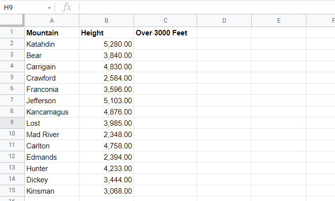
You’re only interested in hiking mountains that are higher than 3000 feet in altitude. So you create another column called “Over 3000 Feet”. An IF statement is the easiest way to fill out this field.

Here’s how an IF statement works:

IF(logical_expression, value_if_true, value_if_false)

The parameters in the IF statement work as follows:

• Logical_expression: This is a conditional statement using operators like <, >, or =.
• Value_if_true: Enter what you want in the cell if the logical expression is TRUE.
• Value_if_false: Enter what you want in the cell if the logical expression is FALSE.

In this example, start with the first row and place the cursor in cell C2. Then, type the following formula:

=IF(B2>3000,”YES”,”NO”)

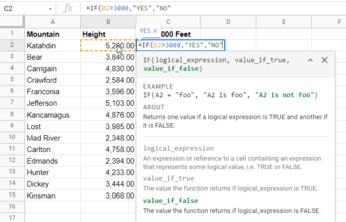
This IF statement means if the height of the mountain in cell B2 is greater than 3000, then display YES in cell C2, otherwise display NO.

Press Enter and you’ll see the correct result (YES) in cell C2.

You may also see a Google Sheets suggestion to autofill the rest of the cells below this one. Select the checkmark if you’d like to go ahead and autofill the rest of the cells with this same function. The references will automatically update to the correct cells for those mountain heights.

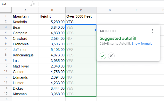
If you don’t see this suggestion, you can hold the Shift key on your keyboard and double-click the small square at the lower right corner of the cell where you entered the first formula.

Using Nested IF Statements in Google Sheets

Now let’s look at an example of creating a nested IF statement in Google Sheets.

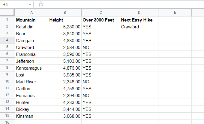
Using the same example as above, let’s say you want to find the first mountain in the list that isn’t over 3,000 feet in altitude so you choose it as your next “easy” hike. To search from top to bottom in a column for the next item that matches a condition requires a nested IF statement.

Place the cursor in the cell where you’d like the result to go. Then, type the following formula:

=IF(B2<3000,A2,IF(B3<3000,A3,IF(B4<3000,A4,IF(B5<3000,A5,IF(B6<3000,A6,IF(B7<3000,A7,IF(B8<3000,A8,IF(B9<3000,A9,IF(B10<3000,A10,IF(B11<3000,A11,IF(B12<3000,A12,IF(B13<3000,A13,IF(B14<3000,A14,IF(B15<3000,A15,”None”))))))))))))))

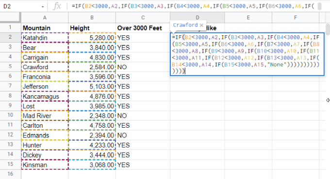
Looks a bit crazy, doesn’t it? Yes, nested IF statements can get complicated. Let’s break this one down so it makes more sense.

The first part of the statement (=IF(B2<3000) checks if the first cell in the column is less than 3000. If it is, then that’s the first mountain on the list under 3000 and so it will return A2 (,A2) since that IF statement is true. 

If it’s false, then you need to nest another IF statement to check the next column (,IF(B3<3000). If this is true, return A3 (,A3)

You repeat this nesting of IF statements until you get all the way down to A15, and then close out all of the if statements with the repeated “)” character.

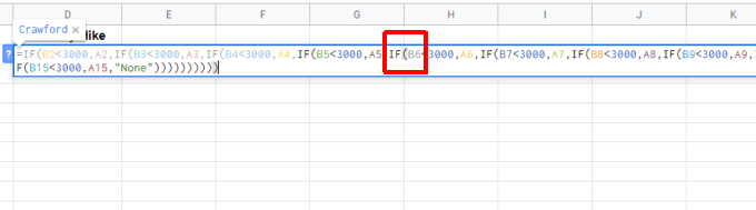
You’ll notice the last “false” parameter in the nested IF statement is “None”. This is because if A15 isn’t under 3000 feet either, then none of the mountains are under 3000 feet.

In this example, here’s what the result will look like in cell D2.

Pro-tip: A simpler way to do this is to use the INDEX, MATCH, and VLOOKUP functions.

Nested IF Statement to Find the Highest Number

In the previous example, the IF statements were nested as FALSE parameters inside the IF statement before it. An opposite example of nesting IF statements is nesting them as TRUE parameters.

You may use this approach to find the highest number in a list. For example, let’s say you have a list of students and their test grades. You want to use nested IF statements to find the highest grade.

Place the cursor in the cell where you want to place the result and type the following formula:

=IF(B2>B3,IF(B2>B4,B2,IF(B4>B3,B4,B3)),B3)

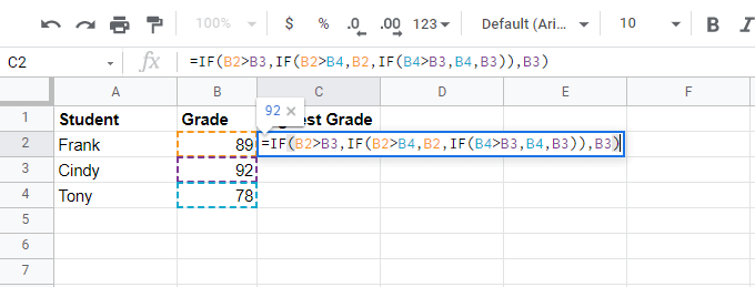
The first part of the statement (=IF(B2>B3) checks if the first cell in the column is greater than the second. If it is, then that cell (B2) may be the largest, but you still need to check the rest. So in place of the TRUE parameter, you’ll nest another IF statement checking B2 against B4. 

• If B2 is still larger than B4, it’s the largest number and you can return B2 as the next TRUE parameter. 
• If it isn’t, B4 could be the largest number. So the FALSE parameter needs to check B4 against B3. If it is larger, then it’s the largest number and this final IF statement will return B4 in the TRUE parameter. 
• If it isn’t, then B3 is the largest and should be returned as the final FALSE parameter. 
• Finally, if the second check (B2>B4) is false, then B3 is the largest because the first IF statement (B2>B3) is already false, so B3 can be returned as this FALSE parameter.

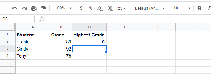
Here’s what the result looks like:

Confused yet?

You’re not alone. Using nested IF statements for something like this is pretty complicated. And once you add even more numbers to the list, it gets even more complex.

That’s why Google Sheets actually has a MAX function where you simply pass it the range of cells (in this case the column), and it’ll return the maximum number. There’s also a MIN function that will return the minimum value.

A Realistic Nested IF Google Sheets Example

The previous two examples were intended to show you how easy it is to get into a mess if you use nested IF statements when you really shouldn’t. That’s an easy trap to get into. Always look for a simpler, single Google Sheets function to accomplish what you’re trying to do.

For example, let’s say you own a company and you’ve received feedback about four employees. Based on the four characteristics that you received feedback on, you need to determine if each employee is promotion material.

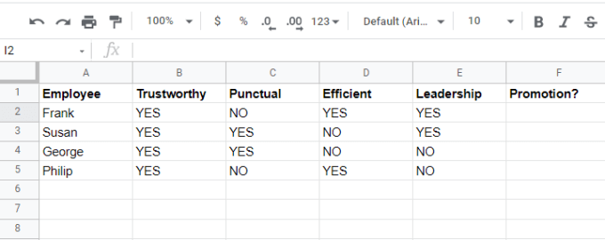
You can write a nested IF statement that’ll examine the answer for each characteristic and then provide a decision in the result column.

If the employee wasn’t:

• Punctual: You’re not too concerned, but you may not promote (maybe not).
• Efficient: You’re not too concerned, and may still promote (maybe).
• Leadership Quality: You may not promote if you agree with the feedback (maybe not).
• Trustworthy: You definitely don’t want to promote (definitely not).

You can program these decisions into the nested IF statement. Place the cursor into the cell where you want the results and type the following formula:

=IF(B2=”YES”,IF(C2=”YES”,IF(D2=”YES”,IF(E2=”YES”,”Definitely”,”Maybe Not”),”Maybe”),”Maybe Not”),”Definitely Not”)

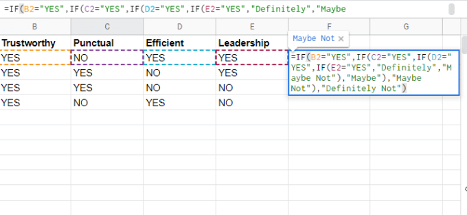
This is a simple nested IF statement that returns “Definitely” if all responses are “YES”, but then returns different answers depending on whether any of the individual cells are “NO”.

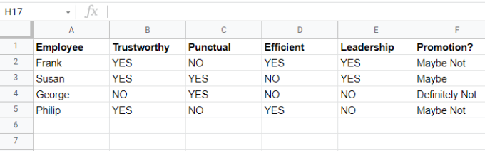
This is one of the few examples where a nested IF statement would be a good choice. But as mentioned above, if you need to do anything much more complex, you’re much better off looking for an existing Google Sheets function that accomplishes the same goal much easier. 

Some examples of great advanced “IF” functions include SUMIF, COUNTIFS, SUMIFS, and AVERAGEIFS.