If you’re tasked with calculating mean for a group of numbers, you can do so in just minutes using Microsoft Excel. With the AVERAGE function, you can find the arithmetic mean, which is average, using a simple formula.
We’ll show you several examples of how you can use the AVERAGE function to do this. These can accommodate most any data set and will help with your data analysis.
What is Mean?
Mean is a statistical term used to explain a set of numbers and has three forms. You can calculate the arithmetic mean, geometric mean, or harmonic mean.
For this tutorial, we’ll explain how to calculate the arithmetic mean which is known in math as the average.
To obtain the result, you sum your group of values and divide the result by the number of values. As an example, you can use these equations to find the average, or mean, for numbers 2, 4, 6, and 8:
=(2+4+6+8)/4
=20/4
=5
As you can see, you first add 2, 4, 6, and 8 to receive the total of 20. Then, divide that total by 4, which is the number of values you just summed. This gives you a mean of 5.
About the AVERAGE Function
In Excel, the AVERAGE function is considered a summary function, and it allows you to find the mean for a set of values.
The syntax for the formula is “AVERAGE(value1, value2,…)” where the first argument is required. You can include up to 255 numbers, cell references, or ranges as arguments.
You also have the flexibility to include a combination of numbers, references, or ranges in the formula.
Something to keep in mind when using the AVERAGE function is that blank cells are not the same as cells with zeros. To avoid skewing your formula’s result, enter zeros in any empty cells if the intended value there is zero.
Text values can give you incorrect results as well, so be sure to only use numeric values in the cells referenced in the formula. As an alternative, you can check out the AVERAGEA function in Excel.
Let’s look at some examples for calculating mean with the AVERAGE function in Excel.
Use the Sum Button to Average Numbers
One of the easiest ways to enter the formula for the AVERAGE function is using a simple button. Excel is smart enough to recognize the numbers you want to use, giving you a quick mean calculation.
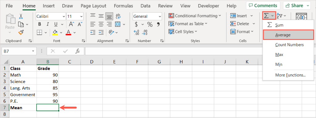
- Select the cell where you want the average (mean).
- Go to the Home tab and open the Sum drop-down list in the Editing section of the ribbon.
- Choose Average from the list.
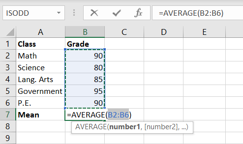
- You’ll see the formula appear in your cell with what Excel believes you want to calculate.
- If this is correct, use Enter or Return to accept the formula and view your result.
If the suggested formula isn’t correct, you can adjust it using one of the options below.
Create a Formula With the AVERAGE Function
Using the syntax described earlier, you can manually create the formula for the AVERAGE function for numbers, references, ranges, and combinations.
Create a Formula for Numbers
If you want to enter the numbers that you want the mean for, you simply type them into the formula as arguments. Be sure to separate the numbers with commas.
Using this formula, we’ll get the average for numbers 10, 20, 30, and 40:
=AVERAGE(10,20,30,40)
Use Enter or Return to receive your result in the cell with the formula, which for this example is 25.
Create a Formula with Cell References
To obtain the mean for values in cells, you can either select the cells or type the cell references in the formula.
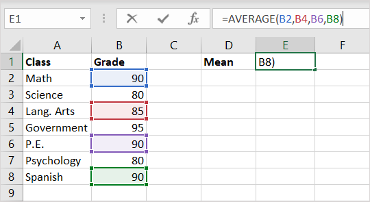
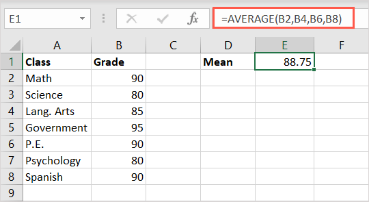
Here, we’ll get the average for cells B2, B4, B6, and B8 with this formula followed by Enter or Return:
=AVERAGE(B2,B4,B6,B8)
You can type the equal sign, function and opening parenthesis. Then, just select each cell to place it into the formula and add the closing parenthesis. Alternatively, you can type the cell references with a comma between each.
Again, you’ll immediately see your result in the cell containing the formula.
Create a Formula for Cell Ranges
Maybe you want the mean for a range of cells or groups of ranges. You can do this by selecting or entering the ranges separated by commas.
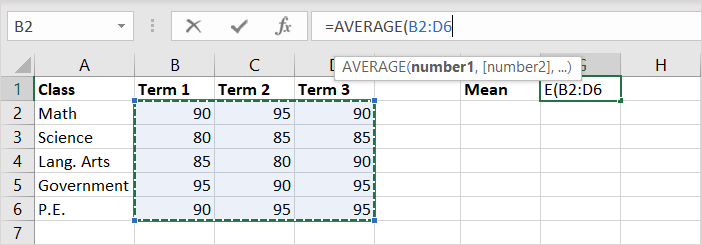
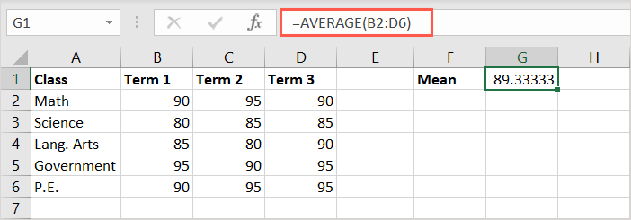
With the following formula, you can calculate the average for cells B2 through D6:
=AVERAGE(B2:B6)
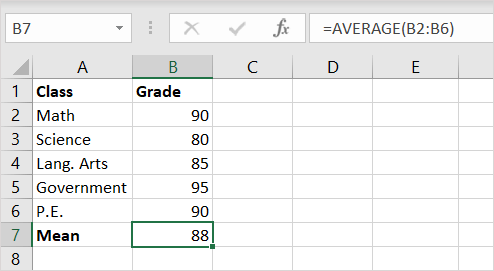
Here, you can type the equal sign, function and opening parenthesis, then simply select the cell range to pop it into the formula. Again, you can enter the range manually if you prefer.
You’ll then receive your result.
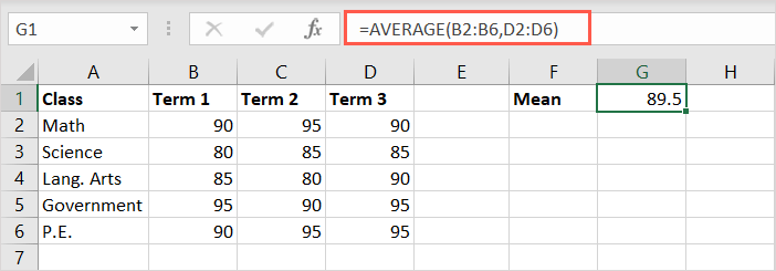
Using this next formula, you can calculate the average for the cell ranges B2 through B6 and D2 through D6:
=AVERAGE(B2:B6,D2:D6)
You’ll then receive your result in the cell with the formula.
Create a Formula for a Combination of Values
For one final example, you might want to calculate the mean for a combination of ranges, cells, and numbers.
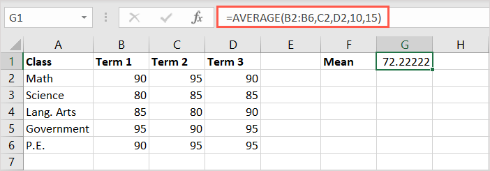
Here, we’ll find the average for cells B2 through B6, C2 and D2, and the numbers 10 and 15 using this formula:
=AVERAGE(B2:B6,C2,D2,10,15)
Just like the formulas above, you can use a mixture of selecting the cells and typing the numbers.
Add the closing parenthesis, use Enter or Return to apply the formula, and then view your result.
View the Average at a Glance
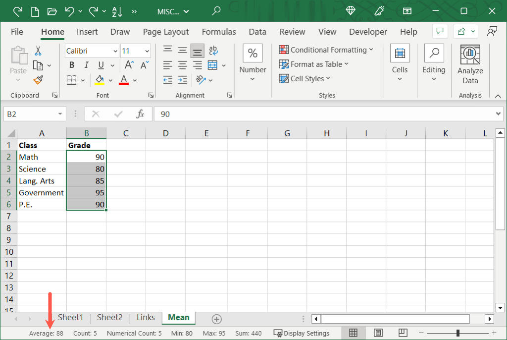
One more Excel tip worth mentioning is ideal if you want to find the mean but not necessarily place the average formula and result in your spreadsheet. You can select the cells you want to calculate and look down at the Status Bar for the Average.
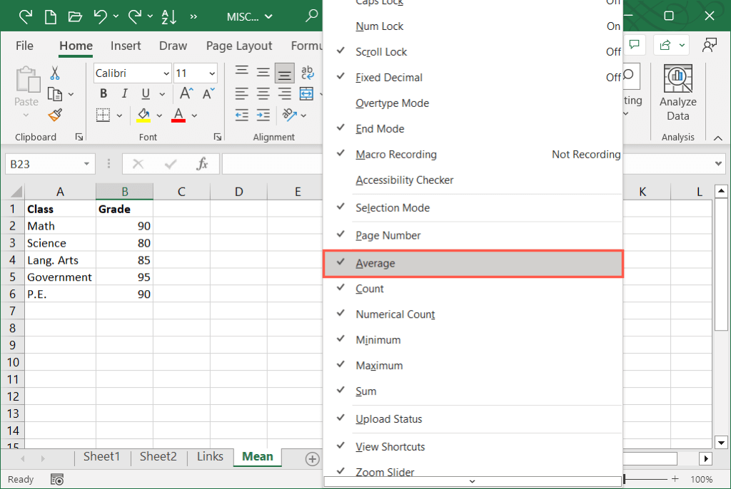
First, make sure you have the calculation enabled. Right-click the Status Bar (below the tab row) and confirm that Average is checked.
Then, simply select the cells you want to average and look to the Status Bar for the result.
When you need to find the mean in Excel, the AVERAGE function saves the day. You don’t have to dig out your calculator, just use one of these methods to get the result you need.
For related tutorials, look at how to use the AVERAGEIFS function in Excel for averaging values with multiple criteria.
Related Posts
Sandy Writtenhouse is a freelance technology writer and former Project, Department, and Program Manager. She turned her education, job experience, and love of technology into a full-time writing career. With all sorts of gadgets in her home and her hands, she seeks to help others make life easier through technology. Read Sandy’s Full Bio


